Automated Detection of Seasonal Epidemic Onset in R • aedseo

library(aedseo)
library(tibble)
library(tidyr)
library(dplyr)
library(ggplot2)

Introduction

The methodology used to detect the onset of seasonal respiratory epidemics can be divided into two essential criteria:

The local estimate of the exponential growth rate, \(r\), is significantly greater than zero.
The sum of cases (SoC) over the past \(k\) units of time exceeds a disease-specific threshold.

Here, \(k\) denotes the window size employed to obtain the local estimate of the exponential growth rate and the SoC. When both of these criteria are met, an alarm is triggered and the onset of the seasonal epidemic is detected.

Exponential growth rate

The exponential growth rate, denoted as \(r\), represents the per capita change in the number of new cases per unit of time. Given that incidence data are integer-valued, the proposed method relies on generalized linear models (GLM). For count data, the Poisson distribution is a suitable choice as a model. Hence, the count observations denoted as \(Y\) are assumed to follow a Poisson distribution

\[\begin{equation} Y \sim \mathrm{Pois}(\lambda) \end{equation}\]

Here, the link function, \(\log()\), connects the linear predictor to the expected value of the data point, expressed as \(\log(\lambda)=\mu\). Given a single continuous covariate \(t\), the mean \(\mu\) can be expressed as

\[\begin{equation} \mu = \alpha + r t \end{equation}\]

This is equivalent to a multiplicative model for \(\lambda\), i.e.

\[\begin{equation} \lambda = \exp(\alpha + r t) = \exp(\alpha) \exp(r t) \end{equation}\]

Intuitively, negative values of \(r\) result in a decline in the number of observed cases, while \(r=0\) represents stability, and positive values of \(r\) indicate an increase.

It is important to note that the Poisson distribution assumes that the mean and variance are equal. In reality, real data often deviate from this assumption, with the variance (\(v\)) being significantly larger than the mean. This biological phenomenon, known as overdispersion, can be addressed within a model in various ways. One approach is to employ quasi-Poisson regression, which assumes \(v=\sigma\lambda\), or to use negative binomial regression (not implemented yet), which assumes \(v=\lambda+\lambda^2/\theta\), where both \(\sigma\) and \(\theta\) are overdispersion parameters.

Simulations

To assess the effectiveness of the aedseo function, we simulate some data. The simulated data is generated using a negative binomial model with a mean parameter \(\mu\) and a variance parameter \(\phi\mu\). In this context \(\phi\) denotes a dispersion parameter, which is assumed to be greater than or equal to 1. The mean, denoted as \(\mu(t)\), is defined by a linear predictor that incorporates both a trend component and seasonality components represented by Fourier terms. The equation \(\mu(t)\) is as follows:

\[\begin{equation} \mu(t) = \exp\Biggl( \theta + \beta t + \sum_{j=1}^m \biggl( \gamma_{\sin} \sin\Bigl( \frac{2 \pi t}{52}\Bigl) + \gamma_{\cos} \cos \Bigl( \frac{2 \pi t}{52} \Bigl) \biggl) \Biggl) \end{equation}\]

mu_t <- function(
    t,
    theta = 1,
    exp_beta = 1.001,
    gamma_sin = 1,
    gamma_cos = 1,
    trend = 1,
    j = 1,
    ...) {
  # Start construction of linear predictor
  linear_predictor <- theta
  # ... add a trend if the scenario request it
  if (trend == 1) {
    linear_predictor <- linear_predictor + log(exp_beta) * t
  }
  # ... add a seasonal component
  linear_predictor <- linear_predictor +
    gamma_sin * sin(2 * pi * t * j / 52) + gamma_cos * cos(2 * pi * t * j / 52)

  return(exp(linear_predictor))
}

simulate_from_nbinom <- function(...) {
  # Set some default values for the simulation
  default_pars <- list(
    "t" = 1,
    "theta" = 1,
    "exp_beta" = 1.001,
    "gamma_sin" = 1,
    "gamma_cos" = 1,
    "trend" = 1,
    "j" = 1,
    "phi" = 1,
    "seed" = 42
  )

  # Match call
  mc <- as.list(match.call())[-1]
  # ... and change parameters relative to the call
  index_mc <- !names(default_pars) %in% names(mc)
  mc <- append(mc, default_pars[index_mc])[names(default_pars)]

  # Set the seed
  set.seed(mc$seed)

  # Calculate the number of time points
  n <- length(eval(mc$t))
  # Calculate mu_t
  mu_t_scenario <- do.call(what = "mu_t", args = mc)
  # ... and compute the variance of the negative binomial distribution
  variance <- mu_t_scenario * mc$phi
  # ... and infer the size in the negative binomial distribution
  size <- (mu_t_scenario + mu_t_scenario^2) / variance
  # Plugin and simulate the data
  simulation <- rnbinom(n = n, mu = mu_t_scenario, size = size)

  return(list("mu_t" = mu_t_scenario, "simulation" = simulation, "pars" = mc))
}

# Define the number of years and the number of months within a year
years <- 3
weeks <- 52
# ... calculate the total number of observations
n <- years * weeks
# ... and a vector containing the overall time passed
time_overall <- 1:n
# Create arbitrary dates
dates <- seq.Date(from = as.Date("2010-01-01"), by = "week", length.out = n)


# Simulate the data
simulation <- simulate_from_nbinom(t = time_overall, theta = log(1000), phi = 5)

# Collect the data in a 'tibble'
sim_data <- tibble(
  Date = dates,
  mu_t = simulation$mu_t,
  y = simulation$simulation
)

A total of three years of weekly data are then simulated with the following set of parameters:

\(\theta=\log(1000)\), representing an average intensity of 1000 cases.
\(\exp(\beta)=1.001\), indicating a slowly increasing trend.
\(\gamma_{\sin} = 1\) and \(\gamma_{\cos} = 1\), representing the seasonality component.
\(\phi = 5\), which represents the dispersion parameter for the negative binomial distribution.

Applying the algorithm

In the following section, the application of the algorithm to the simulated data is outlined. The first step is to transform the simulated data into a aedseo_tsd object using the tsd() function.

# Construct an 'aedseo_tsd' object with the time series data
tsd_data <- tsd(
  observed = sim_data$y,
  time = sim_data$Date,
  time_interval = "week"
)

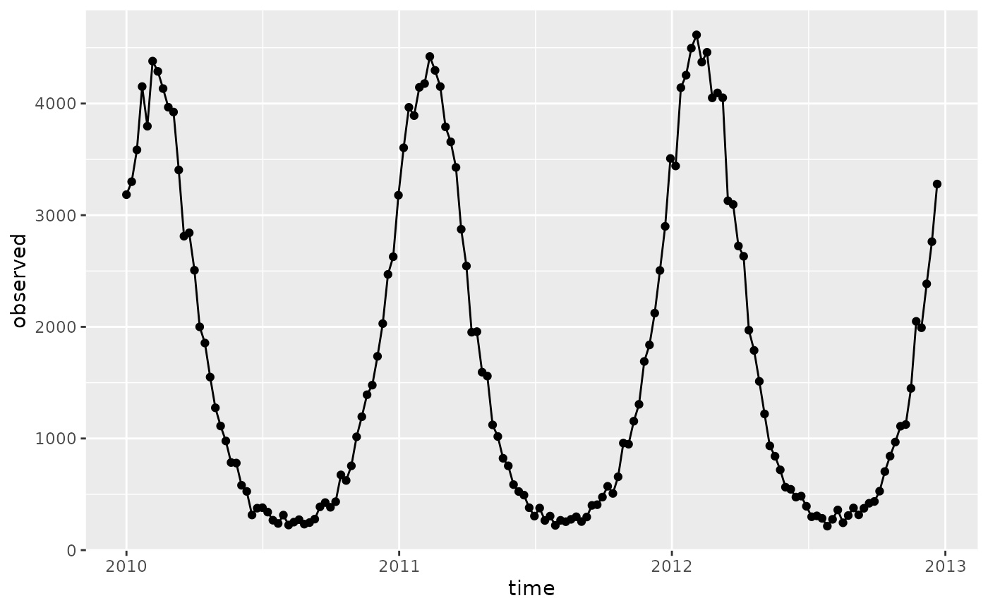
In the following figure, the simulated data (solid circles) is visualized alongside the mean (solid line) for the three arbitrary years of weekly data.

# Have a glance at the time varying mean and the simulated data
plot(tsd_data)

Next, the time series data object is passed to the aedseo() function. Here, a window width of \(k=5\) is specified, meaning that a total of 5 weeks is used in the local estimate of the exponential growth rate. Additionally, a 95% confidence interval is specified. Finally, the exponential growth rate is estimated using quasi-Poisson regression to account for overdispersion in the data.

# Apply the 'aedseo' algorithm
aedseo_results <- aedseo(
  tsd = tsd_data,
  k = 5,
  level = 0.95,
  disease_threshold = 2000,
  family = "quasipoisson"
)

The aedseo package implements S3 methods

In this section, we will explore how to use the plot(), predict() and summary() S3 methods provided by the aedseo package. These methods enhance the functionality of your aedseo objects, allowing you to make predictions and obtain concise summaries of your analysis results.

Visualizing Growth Rates

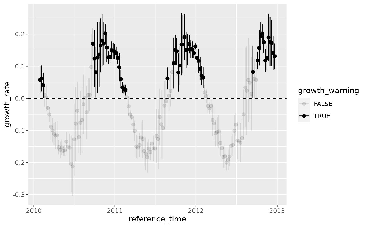
In the figure below, we present the local estimate of the growth rate along with its corresponding 95% confidence interval. This visualization can be generated by utilizing the plot() S3 method specifically designed for objects of the aedseo class.

# Employing the S3 `plot()` method
plot(aedseo_results)

#> Warning: Using alpha for a discrete variable is not advised.

#> Warning: Using alpha for a discrete variable is not advised.

Predicting Growth Rates

The predict method for aedseo objects allows you to make predictions for future time steps based on the estimated growth rates. Here’s how to use it:

# Example: Predict growth rates for the next 5 time steps
(prediction <- predict(aedseo_results, n_step = 5))
#> # A tibble: 6 × 5
#>       t time       estimate lower upper
#>   <int> <date>        <dbl> <dbl> <dbl>
#> 1     0 2012-12-21    3279. 3279. 3279.
#> 2     1 2012-12-22    3736. 3590. 3889.
#> 3     2 2012-12-23    4257. 3930. 4613.
#> 4     3 2012-12-24    4851. 4303. 5471.
#> 5     4 2012-12-25    5527. 4710. 6490.
#> 6     5 2012-12-26    6298. 5157. 7697.

In the example above, we use the predict method to predict growth rates for the next 5 time steps. The n_step argument specifies the number of steps into the future you want to forecast. The resulting prediction object will contain estimates, lower bounds, and upper bounds for each time step.

Summarizing aedseo results

The summary method for aedseo objects provides a concise summary of your automated early detection of seasonal epidemic onset (aedseo) analysis. You can use it to retrieve important information about your analysis, including the latest growth warning and the total number of growth warnings:

summary(aedseo_results)
#> Summary of aedseo Object
#> 
#>     Called using distributional family:
#>       quasipoisson
#> 
#>     Window size for growth rate estimation and
#>     calculation of sum of cases:
#>       5
#> 
#>     Disease specific threshold:
#>       2000
#> 
#>     Reference time point:
#>       2012-12-21
#> 
#>     Sum of cases at reference time point:
#>       12468
#>     Latest sum of cases warning:
#>       2012-12-21
#> 
#>     Growth rate estimate at reference time point:
#>       Estimate   Lower (2.5%)   Upper (97.5%)
#>          0.131     0.091          0.171
#> 
#>     Total number of growth warnings in the series:
#>       59
#>     Latest growth warning:
#>       2012-12-21
#> 
#>     Latest seasonal onset alarm:
#>       2012-12-21

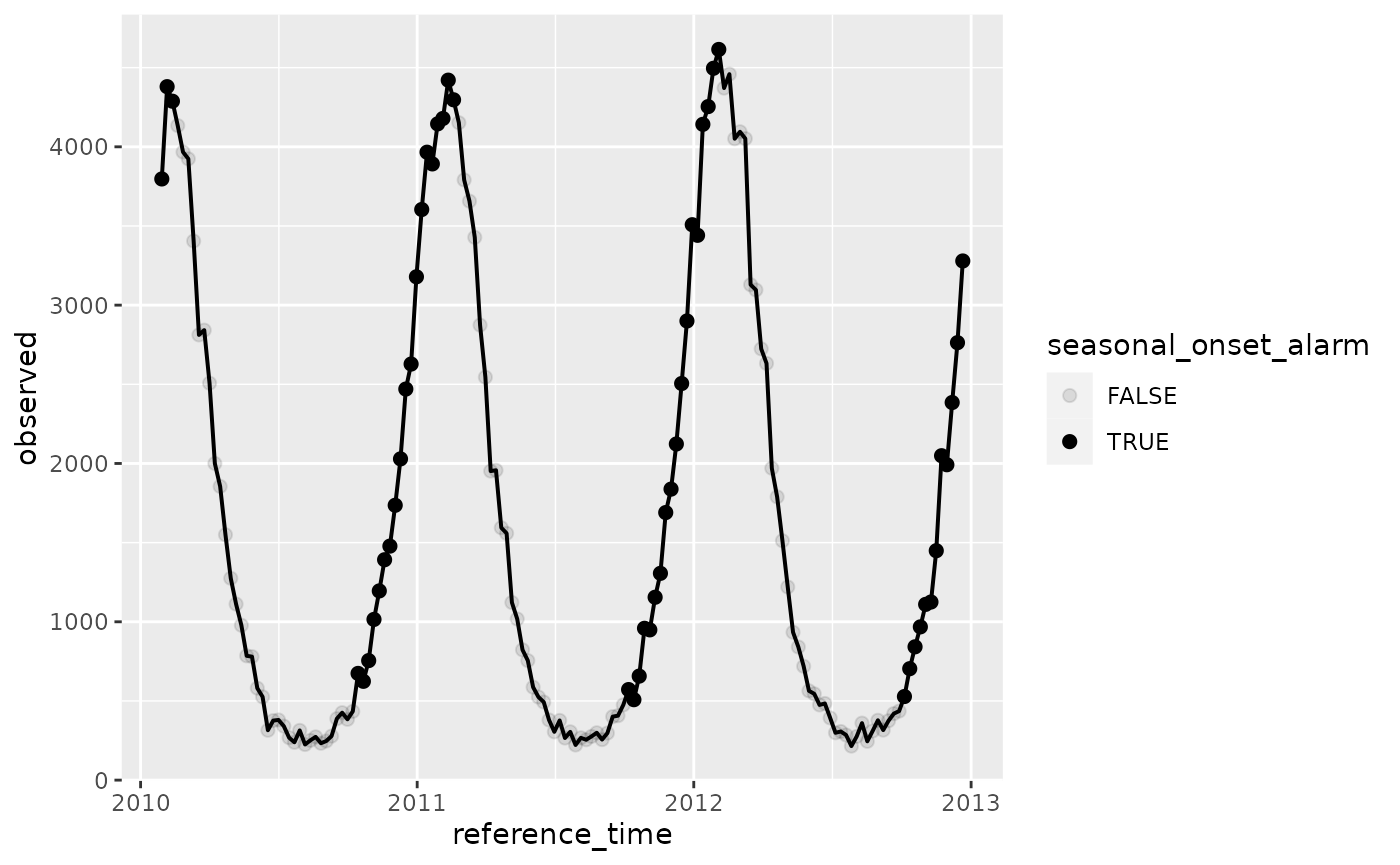
The summary method generates a summary message that includes details such as the reference time point, growth rate estimates, and the number of growth warnings in the series. It helps you quickly assess the key findings of your analysis.