Seasonal Burden Levels

library(aedseo)

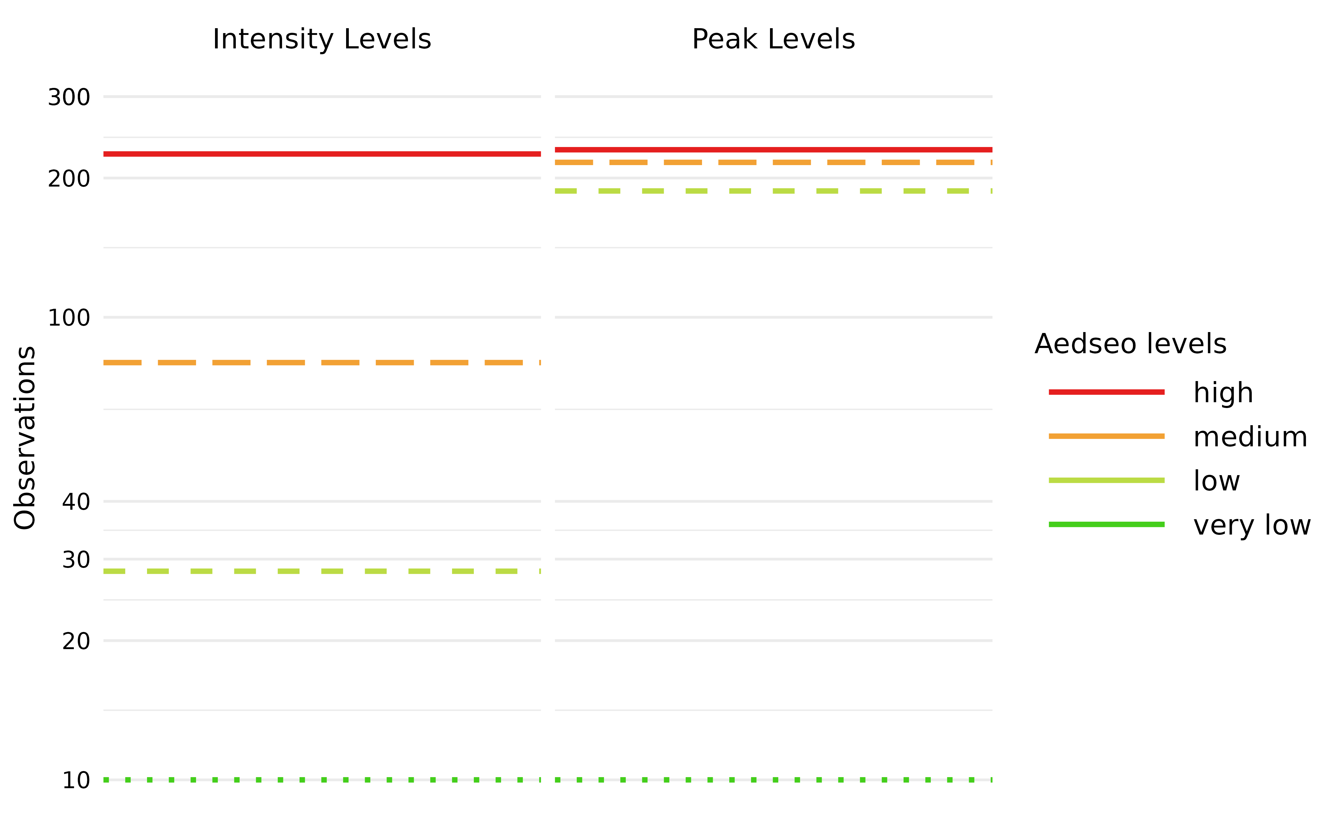
To provide a concise overview of how the seasonal_burden_levels() algorithm operates, we utilize the same example data presented in the vignette("aedseo"). The plot below illustrates the two methods available for estimating burden levels in the combined_seasonal_output() function:

• intensity_levels: Intended for within-season classification of observations.
• peak_levels: Intended for comparing the height of peaks between seasons.

The disease-specific threshold is the very low breakpoint for both methods. Breakpoints are named as the upper bounds for the burden levels, and are visualised on following plot.

Methodology

The methodology used to define the burden levels of seasonal epidemics is based on observations from previous seasons. Historical data from all available seasons is used to establish the levels for the current season. This is done by:

• Using n highest (peak) observations from each season.
• Selecting only observations if they surpass the disease-specific threshold.
• Weighting the observations such that recent observations have a greater influence than older observations.
• A proper distribution (log-normal, weibull and exponential are currently implemented) is fitted to the weighted n peak observations. The selected distribution with the fitted parameters is used to calculate percentiles to be used as breakpoints.
• Burden levels can be defined by two methods:
  • peak_levels which models the height of the seasonal peaks. Using the log-normal distribution without weights is similar to the default in mem.
  • intensity_levels which models the within season levels. The highest breakpoint is identical with the peak_levels method. Intermediate breakpoints are evenly distributed on a logaritmic scale, between the very low and high breakpoints, to give the same relative difference between the breakpoints.

The model is implemented in the seasonal_burden_levels() function of the aedseo package. In the following sections we will describe the arguments for the function and how the model is build.

Peak observations

The n_peak argument defines the number of highest observations to be included from each season. The default of n_peak is 6 - corresponding with the mem defaults of using 30 observations across the latest five seasons.

Weighting

The decay_factor argument is implemented to give more weight to recent seasons, as they are often more indicative of current and future trends. As time progresses, the relevance of older seasons may decrease due to changes in factors like testing recommendations, population immunity, virus mutations, or intervention strategies. Weighting older seasons less reflects this reduced relevance. From time-series analysis, $\frac{1}{1-\text{decay_factor}}$ is often used as an approximate “effective memory”. Hence, with the default decay_factor = 0.8 the effective memory is five seasons. (See mentioned by Hyndman & Athanasopoulos for an introduction to simple exponential smoothing) The default decay_factor allows the model to be responsive to recent changes without being overly sensitive to short-term fluctuations. The optimal decay_factor can vary depending on the variability and trends within the data. For datasets where seasonal patterns are highly stable, a higher decay_factor (i.e. longer memory) may be appropriate. Conversely, if the data exhibit dramatic shifts from one season to the next, a lower decay_factor may improve predictions.

Distribution and optimisation

The family argument is used to select which distribution the n_peak observations should be fitted to, users can choose between lnorm, weibull and exp distributions. The log-normal distribution theoretically aligns well with the nature of epidemic data, which often exhibits multiplicative growth patterns. In our optimisation process, we evaluated the distributions to determine their performance in fitting Danish non-sentinel cases and hospitalisation data for RSV, SARS-CoV-2 and Influenza (A and B). All three distributions had comparable weighted likelihood values during optimisation, hence we did not see any statistical significant difference in their performance.

The model uses the fit_percentiles() function which employs the stats::optim for estimating the parameters that maximizes the weighted likelihood. The optim_method argument can be passed to seasonal_burden_levels(), default is Nelder-Mead but other methods can be selected, see ?fit_percentiles.

Burden levels

The method argument is used to select one of the two methods intensity_levels(default) and peak_levels. Both methods return percentile(s) from the fitted distribution which are used to define the breakpoins for the burden levels. Breakpoints are named very low, low, medium and high and define the upper bound of the corresponding burden level.

• intensity_levels takes one percentile as argument, representing the highest breakpoint. The default is set at a 95% percentile. The disease-specific threshold determines the very low breakpoint. The low and medium breakpoints are calculated to give identical relative increases between the very low and high breakpoints.

• peak_levels takes three percentiles as argument, representing the low, medium and high breakpoints. The default percentiles are 40%, 90%, and 97.5% to align with the parameters used in mem. The disease-specific threshold defines the very low breakpoint.

Applying the seasonal_burden_levels() algorithm

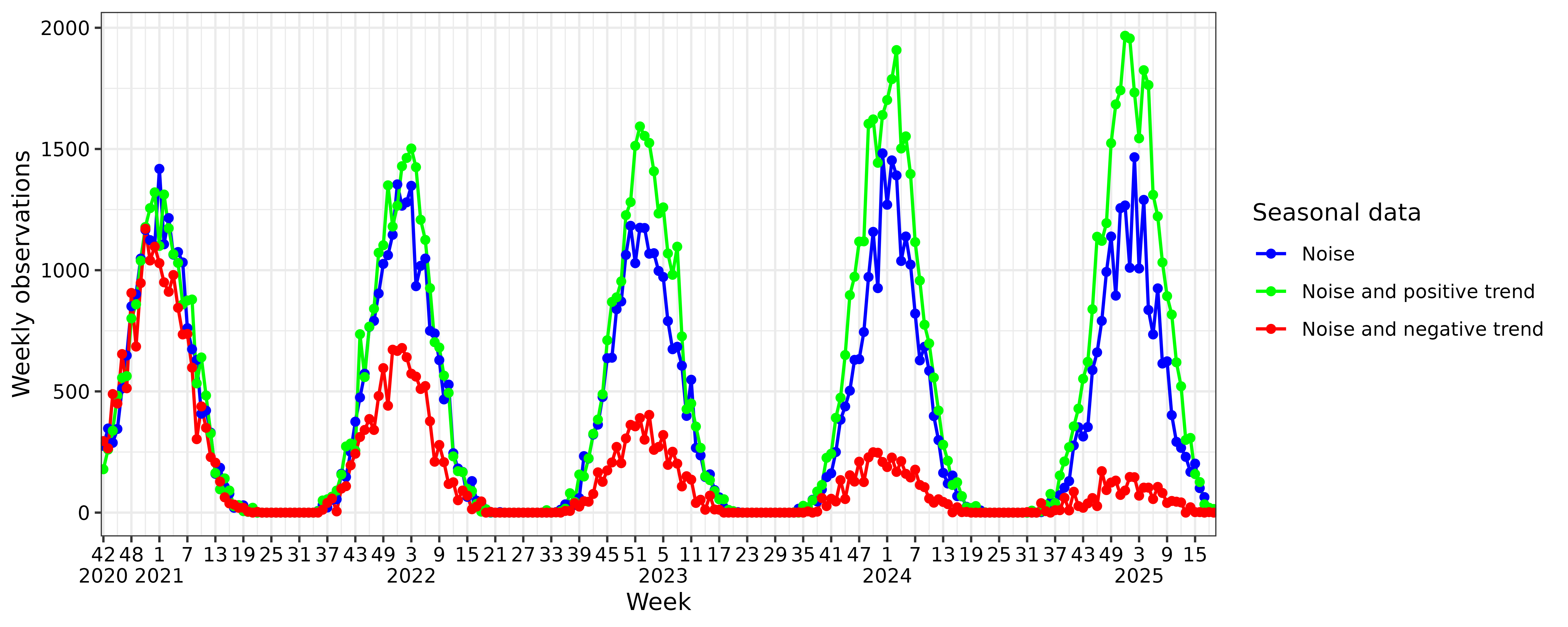
The same data is created with following combinations:

• noise
• noise and positive trend
• noise and negative trend

These combinations are selected as it is realistic for real world data to have noise, and differentiation between trend can occur declining or inclining between seasons. Breakpoints for season 2024/2025 are calculated based on the three previous seasons.

To apply the seasonal_burden_levels() algorithm, data needs to be transformed into a tsd object. The disease-specific threshold is determined for all data combinations with use of the method described in vignette("aedseo"). The disease-specific threshold should be revised before a new season starts, especially if the data has a trend.

Use the intensity_levels method

The seasonal_burden_levels() function provides a tsd_burden_level object, which can be used in the summary() S3 method. This provides a concise summary of your comprehensive seasonal burden level analysis, including breakpoints for the current season.

intensity_levels_n <- seasonal_burden_levels(
  tsd = tsd_data_noise,
  disease_threshold = 10,
  method = "intensity_levels",
  conf_levels = 0.975
)
summary(intensity_levels_n)
#> Summary of tsd_burden_levels object
#> 
#>     Breakpoint estimates:
#>       very low : 10.000000
#>       low: 53.267535
#>       medium: 283.743033
#>       high: 1511.429206
#> 
#>     The season for the burden levels:
#>       2025/2026
#> 
#>     Model settings:
#>       Disease specific threshold: 10
#>       Called using distributional family: lnorm

Use the peak_levels method

mem uses the n highest observations from each previous epidemic period to fit the parameters of the distribution, where n = 30/seasons. The data has four previous seasons, to align with mem, we use n_peak = 8

peak_levels_n <- seasonal_burden_levels(
  tsd = tsd_data_noise,
  disease_threshold = 10,
  method = "peak_levels",
  conf_levels = c(0.4, 0.9, 0.975),
  n_peak = 8
)
summary(peak_levels_n)
#> Summary of tsd_burden_levels object
#> 
#>     Breakpoint estimates:
#>       very low : 10.000000
#>       low: 1133.397742
#>       medium: 1366.530366
#>       high: 1484.312479
#> 
#>     The season for the burden levels:
#>       2025/2026
#> 
#>     Model settings:
#>       Disease specific threshold: 10
#>       Called using distributional family: lnorm

Compare intensity_levels, peak_levels and mem algorithms

mem is run with default arguments.

# Remove current season such as previous seasons predict for newest season
previous_seasons <- tsd_data_all |>
  dplyr::mutate(season = epi_calendar(time)) |>
  dplyr::filter(season != "2024/2025") |>
  dplyr::select(-season)

# Run mem algorithm
mem_thresholds <- previous_seasons |>
  dplyr::group_by(Data) |>
  dplyr::group_modify(~ {
    mem_data <- .x |>
      dplyr::mutate(season = aedseo::epi_calendar(time),
                    week = lubridate::isoweek(time)) |>
      dplyr::select(-time) |>
      tidyr::pivot_wider(names_from = season, values_from = observation) |>
      dplyr::select(-week)
    # Run mem
    mem_result <- mem::memmodel(mem_data)
    # Extract thresholds
    mem_thresholds <- tibble::tibble(
      `epidemic threshold \n (mem)` = mem_result$epidemic.thresholds[1],
      `medium` = mem_result$intensity.thresholds[1],
      `high` = mem_result$intensity.thresholds[2],
      `very high` = mem_result$intensity.thresholds[3]
    )
  })

aedseo and mem levels

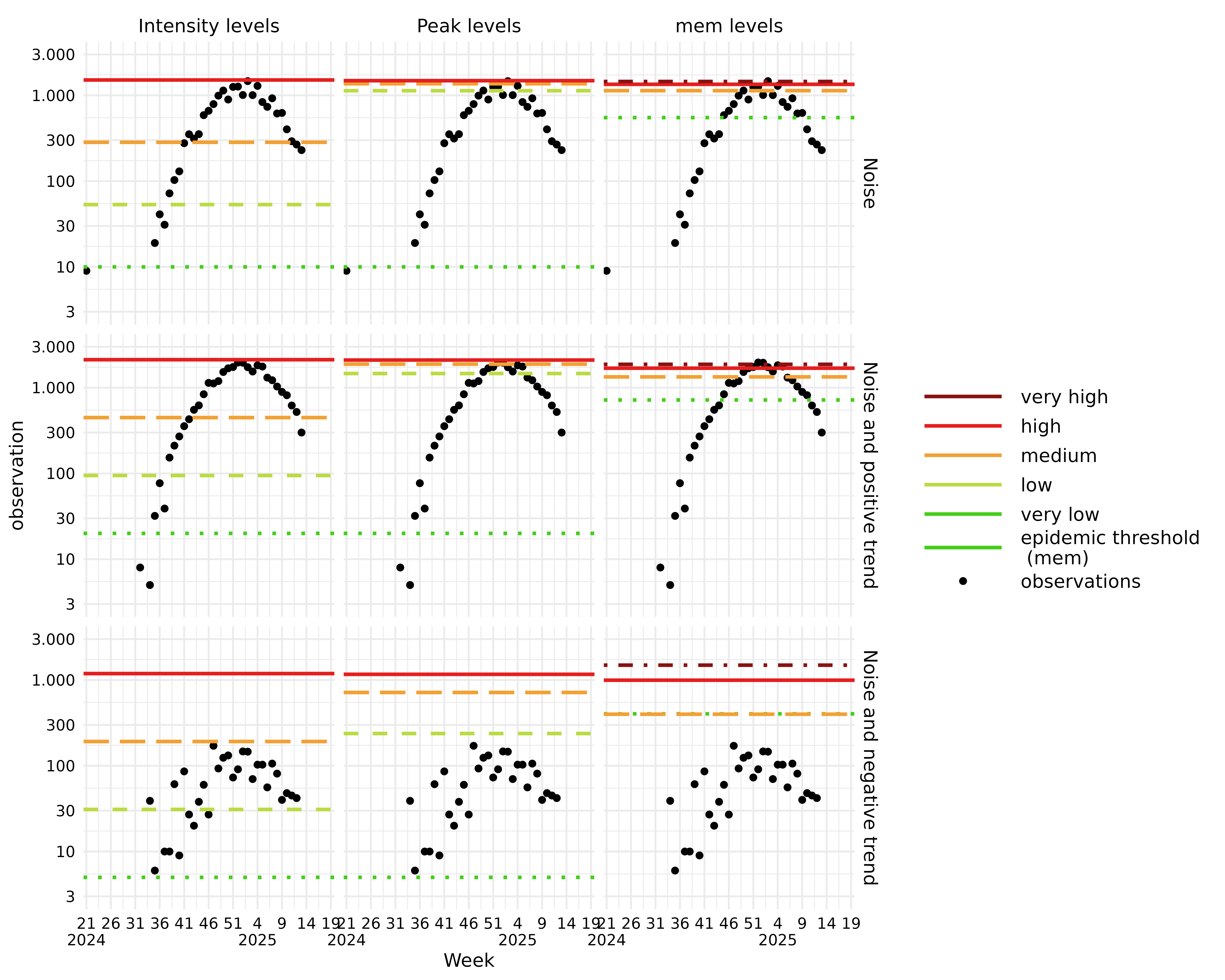
In the plots:

• Observations below 3 are filtered out to improve visualization.
• y scale is log transformed.

Upon examining all methods and data combinations, it becomes clear that the intensity_levels approach establishes levels covering the entire set of observations from previous seasons. In contrast, the peak_levels and mem methods define levels solely based on the highest observations within each season, and are thus only relevant for comparing the height of peaks between seasons.

The highest observations for the 2024/2025 season for each data set are:

Data	Observation
Noise	1466
Noise and positive trend	1967
Noise and negative trend	171

In relation to these highest observations and upon further examination, we observe the following:

Plots with Noise and Noise with Positive Trend:

• Both peak_levels and mem estimate very high breakpoints. This occurs because observations remain consistently elevated across all three seasons, causing these methods to overlook the remaining observations.

Data with Noise and Positive Trend:

• All three methods exhibit higher breakpoints, indicating that they successfully capture the exponentially increasing trend between seasons.

Data with Noise and Negative Trend:

• As observations exponentially decrease between seasons (with the highest observation this season being 171), we expect the breakpoints to be the lowest of these examples. This expectation is met across all three methods. However, the weighting of seasons in intensity_levels and peak_levels leads to older seasons having less impact on the breakpoints, as we progress forward in time. On the other hand, mem includes all high observations from the previous 10 seasons without diminishing the importance of older seasons, which results in sustained very high breakpoints.

• Notably, in the mem method, the epidemic threshold is positioned slightly above the medium burden level. This means that the epidemic period begins only when observations reach the height of the seasonal peaks observed in previous seasons.

In conclusion, the peak_levels and mem methods allows us to compare the height of peaks between seasons, whereas the intensity_levels method supports continuous monitoring of observations in the current season.