DiseasyImmunity optimisation

library(diseasy)
#> Loading required package: diseasystore
#> 
#> Attaching package: 'diseasy'
#> The following object is masked from 'package:diseasystore':
#> 
#>     diseasyoption

im <- DiseasyImmunity$new()

Motivation

From our testing, we have learned that method used to express the waning immunity in a compartmental model¹ is a hard optimisation problem. Depending on the choice of optimisation algorithm, the quality of the approximation will vary wildly as well as the time it takes for the algorithm to converge.

To mitigate this issue, we investigate the effect of several optimisation algorithms to identify the best performing one, evaluating both run time and approximation accuracy of the waning immunity target.

?DiseasyImmunity can internally employ the optimisation algorithms of stats, nloptr and optimx::optimr(), which means that we have around 30 different algorithms to test.

Note that the nature of the optimisation problem also changes dependent on the method used to approximate (i.e. “free_delta”, “free_gamma”, “all_free” - see ?DiseasyImmunity documentation), which means that the algorithm that performs well for one method will not necessarily perform well on the other methods.

Setup

Since we are searching for a “general” best choice of optimisation algorithm, we will define a setup that tests a wide range of waning immunity targets.

We define a “family” of functions to test the optimisation algorithms against. These start at 1 and go to 0 within a time scale, $\tau$.

These targets are:

Function	Functional form
Exponential	$\exp\left(-t / \tau\right)$
Sigmoidal	$\exp\left(-(t - \tau) / 6)\; /\; (1 + \exp\!\!(-(t - \tau) / 6)\right)$
Heaviside	$\Theta(\tau - t)$
Sum of exponentials	$\frac{1}{3}\left(\exp(-t / \tau) + \exp(-2t / \tau) + \exp(-3t / \tau)\right)$
Linear	$\sup\left(\{1 - t/\tau, 0\}\right)$

We then construct more target functions from this family of functions:

• The unaltered functions ($f(t)$)
• The functions but with non-zero asymptote ($g(t) = 0.8 \cdot f(t) + 0.2$)
• The functions but with longer time scales ($h(t) = f(t / 2)$)

The optimisation

As stated above, the optimisation algorithms vary wildly in the time it takes to complete the optimisation. To conduct this test in a reasonable time frame (and to determine algorithms that are reasonably efficient), we setup a testing schema consisting of a number of “rounds” where we incrementally increase the number of compartments in the problem (and thereby the number of degrees of freedom to optimise).

In addition, we allocate a time limit to each algorithm in each round. If the execution time exceeds this time limit, the algorithm is “eliminated” and no more computation is done for the algorithm. Note that this is done on per method basis as we know the optimisation algorithms fare differently on the different methods for approximation.

Once the round is complete, we update the list of eliminated algorithms and the we run the optimisation of $M + 1$ with the reduced set of algorithms.

The entire optimisation process is run both without penalty (monotonous = 0 and individual_level = 0) and with a penalty (monotonous = 1 and individual_level = 1).

The results of the optimisation round in stored in the ?diseasy_immunity_optimiser_results data-set.

results <- diseasy_immunity_optimiser_results

results
#> # A tibble: 37,465 × 10
#>    target  variation      method strategy penalty     M     value execution_time
#>    <chr>   <chr>          <chr>  <chr>    <lgl>   <int>     <dbl>          <dbl>
#>  1 exp_sum Base           all_f… combina… FALSE       2 1.46e-  1        2.92   
#>  2 exp_sum Base           all_f… naive    FALSE       2 1.46e-  1        1.73   
#>  3 exp_sum Base           all_f… recursi… FALSE       2 1.46e-  1        1.69   
#>  4 exp_sum Base           free_… naive    FALSE       2 8.99e+307        0.00725
#>  5 exp_sum Base           free_… recursi… FALSE       2 8.99e+307        0.00647
#>  6 exp_sum Base           free_… naive    FALSE       2 1.46e-  1        1.56   
#>  7 exp_sum Base           free_… recursi… FALSE       2 1.46e-  1        1.56   
#>  8 exp_sum Non-zero asym… all_f… combina… FALSE       2 1.17e-  1        3.00   
#>  9 exp_sum Non-zero asym… all_f… naive    FALSE       2 1.17e-  1        1.58   
#> 10 exp_sum Non-zero asym… all_f… recursi… FALSE       2 1.17e-  1        1.51   
#> # ℹ 37,455 more rows
#> # ℹ 2 more variables: optim_method <chr>, target_label <chr>

Global results

To get an overview of the best performing optimisers, we present an aggregated view of the results in the table below. Here we present the top 5 “best” optimiser/strategy combination for each method and penalty setting. To define what it means to be the “best” we simply take the total integral difference between the approximation and the target function across all target functions and problem sizes ($M$).

Note that we currently filter out the results from the Heaviside and linear targets, which seem to be especially difficult for the optimisers to handle (see the Per target results section below).

In addition, we only consider problems up to size $M = 5$ for the general results.

Table 1: Global results (excluding heaviside and linear targets)

penalty	free_delta			free_gamma			all_free
	strategy	optimiser	value	strategy	optimiser	value	strategy	optimiser	value
no	recursive	bfgs	13.53	recursive	subplex	9.96	combination	neldermead	9.45
no	naive	slsqp	13.53	naive	subplex	10.02	naive	ucminf	9.54
no	naive	tnewton	13.53	naive	pracmanm	10.08	combination	nmkb	9.60
no	naive	ucminf	13.53	naive	uobyqa	10.12	combination	ucminf	9.68
no	recursive	ucminf	13.53	naive	lbfgs	10.15	combination	nelder-mead	9.69
yes	recursive	nelder-mead	15.13	naive	hjkb	11.46	naive	bfgs	10.90
yes	naive	tnewton	15.13	naive	hjn	11.62	naive	ucminf	10.90
yes	naive	ucminf	15.13	recursive	subplex	11.70	naive	newuoa	11.04
yes	recursive	ucminf	15.13	naive	pracmanm	11.71	naive	nmkb	11.35
yes	naive	spg	15.15	naive	subplex	11.71	combination	auglag_cobyla	11.51
auglag_cobyla: auglag with COBYLA as local solver.

To better choose the default optimisers for DiseasyImmunity, we will also consider how fast the different optimisation methods are. For that purpose, we have also measured the time to run the optimisation for each problem.

# Define the defaults for DiseasyImmunity
chosen_defaults <- tibble::tibble(
  "method" = character(0),
  "penalty" = character(0),
  "strategy" = character(0),
  "optim_method" = character(0)
) |>
  tibble::add_row(
    "method" = "free_delta", "penalty" = "no",
    "strategy" = "naive",
    "optim_method" = "ucminf"
  ) |>
  tibble::add_row(
    "method" = "free_delta", "penalty" = "yes",
    "strategy" = "naive",
    "optim_method" = "ucminf"
  ) |>
  tibble::add_row(
    "method" = "free_gamma", "penalty" = "no",
    "strategy" = "naive",
    "optim_method" = "subplex"
  ) |>
  tibble::add_row(
    "method" = "free_gamma", "penalty" = "yes",
    "strategy" = "naive",
    "optim_method" = "hjkb"
  ) |>
  tibble::add_row(
    "method" = "all_free", "penalty" = "no",
    "strategy" = "naive",
    "optim_method" = "ucminf"
  ) |>
  tibble::add_row(
    "method" = "all_free", "penalty" = "yes",
    "strategy" = "naive",
    "optim_method" = "ucminf"
  )

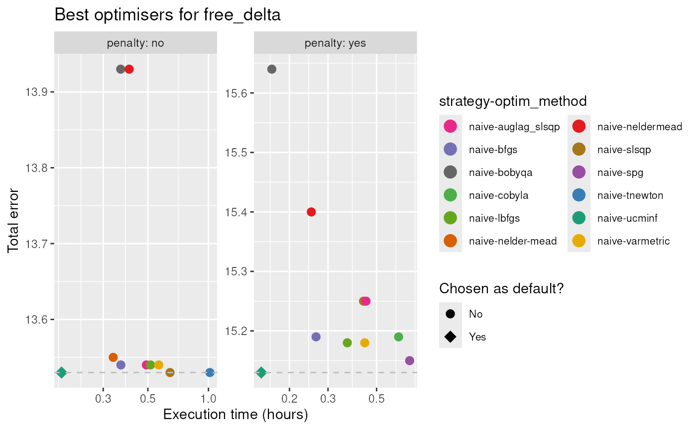
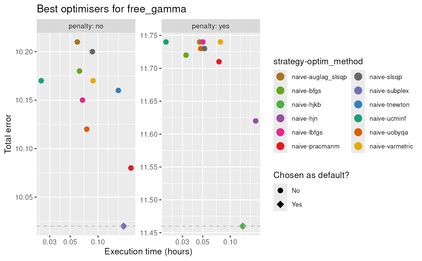
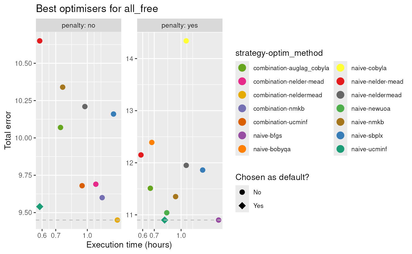
In total, we find that there is no clear choice for best, general optimiser/strategy combination.

For the defaults, we have chose the optimiser/strategy combination dependent on the method of parametrisation and the inclusion of penalty.

The following optimiser/strategy combinations acts as defaults for the ?DiseasyImmunity class:

method	penalty	strategy	optim_method
free_delta	no	naive	ucminf
free_delta	yes	naive	ucminf
free_gamma	no	naive	subplex
free_gamma	yes	naive	hjkb
all_free	no	naive	ucminf
all_free	yes	naive	ucminf

However, as we see in the Per target results section below, the choice of optimiser/strategy can be improved when accounting for the specific target function.

Per target results

Here we dive deeper into the performance of the optimisers on a per target basis. As before, we present best performing optimisers for the given targets in an aggregated view.

We present the top 3 best optimiser/strategy combination for each method and penalty setting.

Table 2: Results for Exponential target

penalty	free_delta			free_gamma			all_free
	strategy	optimiser	value	strategy	optimiser	value	strategy	optimiser	value
no	naive	ucminf	0.00	naive	ucminf	0.00	naive	ucminf	0.00
no	recursive	neldermead	0.00	naive	neldermead	0.00	naive	bobyqa	0.00
no	recursive	nelder-mead	0.00	naive	auglag_slsqp	0.00	naive	neldermead	0.00
yes	naive	ucminf	0.37	recursive	neldermead	0.31	naive	ucminf	0.19
yes	naive	neldermead	0.37	naive	hjkb	0.31	naive	auglag_slsqp	0.19
yes	naive	lbfgs	0.37	naive	hjn	0.31	naive	slsqp	0.19
auglag_lbfgs: auglag with SLSQP as local solver.

Table 3: Results for Sum of exponentials target

penalty	free_delta			free_gamma			all_free
	strategy	optimiser	value	strategy	optimiser	value	strategy	optimiser	value
no	naive	ucminf	0.7	recursive	pracmanm	0.90	naive	pracmanm	0.39
no	naive	bfgs	0.7	recursive	subplex	0.90	combination	neldermead	0.39
no	naive	lbfgs	0.7	naive	subplex	0.93	naive	neldermead	0.43
yes	naive	ucminf	1.6	naive	hjkb	1.38	naive	ucminf	0.94
yes	naive	spg	1.6	naive	hjn	1.44	naive	bfgs	0.94
yes	naive	mla	1.6	recursive	pracmanm	1.51	naive	pracmanm	0.94

Table 4: Results for Sigmoidal target

penalty	free_delta			free_gamma			all_free
	strategy	optimiser	value	strategy	optimiser	value	strategy	optimiser	value
no	naive	ucminf	12.83	naive	auglag_lbfgs	9.06	combination	auglag_cobyla	9.06
no	naive	bobyqa	12.83	naive	uobyqa	9.06	naive	ucminf	9.06
no	naive	lbfgs	12.83	naive	lbfgs	9.06	combination	nmkb	9.06
yes	naive	ucminf	13.16	naive	subplex	9.74	combination	sbplx	9.74
yes	naive	spg	13.16	naive	pracmanm	9.74	combination	bfgs	9.75
yes	naive	bobyqa	13.16	naive	bfgs	9.75	combination	ucminf	9.75
auglag_cobyla: auglag with COBYLA as local solver.
auglag_lbfgs: auglag with LBFGS as local solver.

Table 5: Results for Linear target

penalty	free_delta			free_gamma			all_free
	strategy	optimiser	value	strategy	optimiser	value	strategy	optimiser	value
no	naive	ucminf	5.02	naive	anms	3.91	naive	ucminf	3.92
no	naive	bobyqa	5.02	naive	ucminf	3.92	naive	nelder-mead	3.94
no	naive	lbfgs	5.02	naive	lbfgs	3.92	naive	auglag_cobyla	5.02
yes	naive	auglag_cobyla	5.31	naive	subplex	4.24	combination	pracmanm	4.25
yes	naive	bobyqa	5.31	naive	nmkb	4.25	naive	nmkb	4.26
yes	naive	bfgs	5.31	naive	nelder-mead	4.25	combination	bfgs	4.29
auglag_cobyla: auglag with COBYLA as local solver.

Table 6: Results for Heaviside target

penalty	free_delta			free_gamma			all_free
	strategy	optimiser	value	strategy	optimiser	value	strategy	optimiser	value
no	naive	uobyqa	25.64	naive	nmkb	23.04	naive	ucminf	23.04
no	naive	ucminf	25.64	naive	nelder-mead	23.04	naive	nelder-mead	23.04
no	naive	auglag_cobyla	25.64	naive	ucminf	23.04	naive	auglag_cobyla	24.63
yes	naive	ucminf	25.95	naive	nmkb	23.60	naive	hjn	23.60
yes	naive	bobyqa	25.95	naive	ucminf	23.60	naive	ucminf	23.60
yes	naive	spg	25.95	naive	nelder-mead	23.60	naive	newuoa	23.71
auglag_cobyla: auglag with COBYLA as local solver.