DiseasyModelRegression

library(diseasy)
#> Loading required package: diseasystore
#> 
#> Attaching package: 'diseasy'
#> The following object is masked from 'package:diseasystore':
#> 
#>     diseasyoption

Introduction

In diseasy we bundle some simple regression model templates and provide the tools to create custom regression model templates.

Overview

These are structured as R6 classes that uses inheritance to simplify the creating of individual templates.

Structurally, R6 classes we provide are as follows:

Module	Description
?DiseasyModel	All model templates initially inherit from this module (see vignette("creating-a-model")).
?DiseasyModelRegression	Defines the structure of regression model templates (i.e. must implement $fit_regression(), $get_prediction(), and $update_formula()).
?DiseasyModelGLM	Implements $fit_regression() and $get_prediction() using stats::glm
?DiseasyModelBRM	Implements $fit_regression() and $get_prediction() using brms::brm
?DiseasyModelG0	Implements $update_formula() to create a constant predictor model (from ?DiseasyModelGLM)
?DiseasyModelG1	Implements $update_formula() to create a exponential growth predictor model (from ?DiseasyModelGLM)
?DiseasyModelB0	Implements $update_formula() to create a constant predictor model (from ?DiseasyModelBRM)
?DiseasyModelB1	Implements $update_formula() to create a exponential growth predictor model (from ?DiseasyModelBRM)

Examples

Here we show how to use the simple regression model templates in diseasy.

The regression models are “duplicated” in the sense that there exist two similar models implemented in different statistical engines. The predictions from the models are very similar.

Engine \ model	constant	exponential
glm	?DiseasyModelG0	?DiseasyModelG1
brms	?DiseasyModelB0	?DiseasyModelB1

For the examples below, we therefore show the results from the GLM class of models only.

The data to model

As our example data, we will use the bundled example data ?DiseasystoreSeirExample.

# Configure a observables module with the example data and database
observables <- DiseasyObservables$new(
  diseasystore = DiseasystoreSeirExample,
  conn = DBI::dbConnect(RSQLite::SQLite())
)

The data is stratified by age and covers a single infection wave. It contains two observables of interest for our example:

• n_positive: The observed subset of infected (65% of true infected with weekday variation in detection).
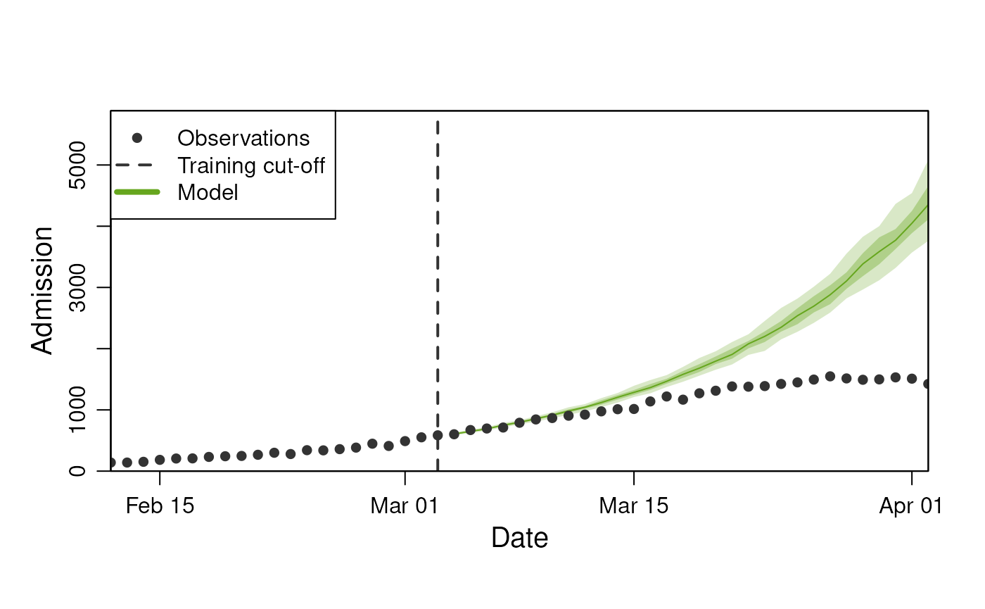
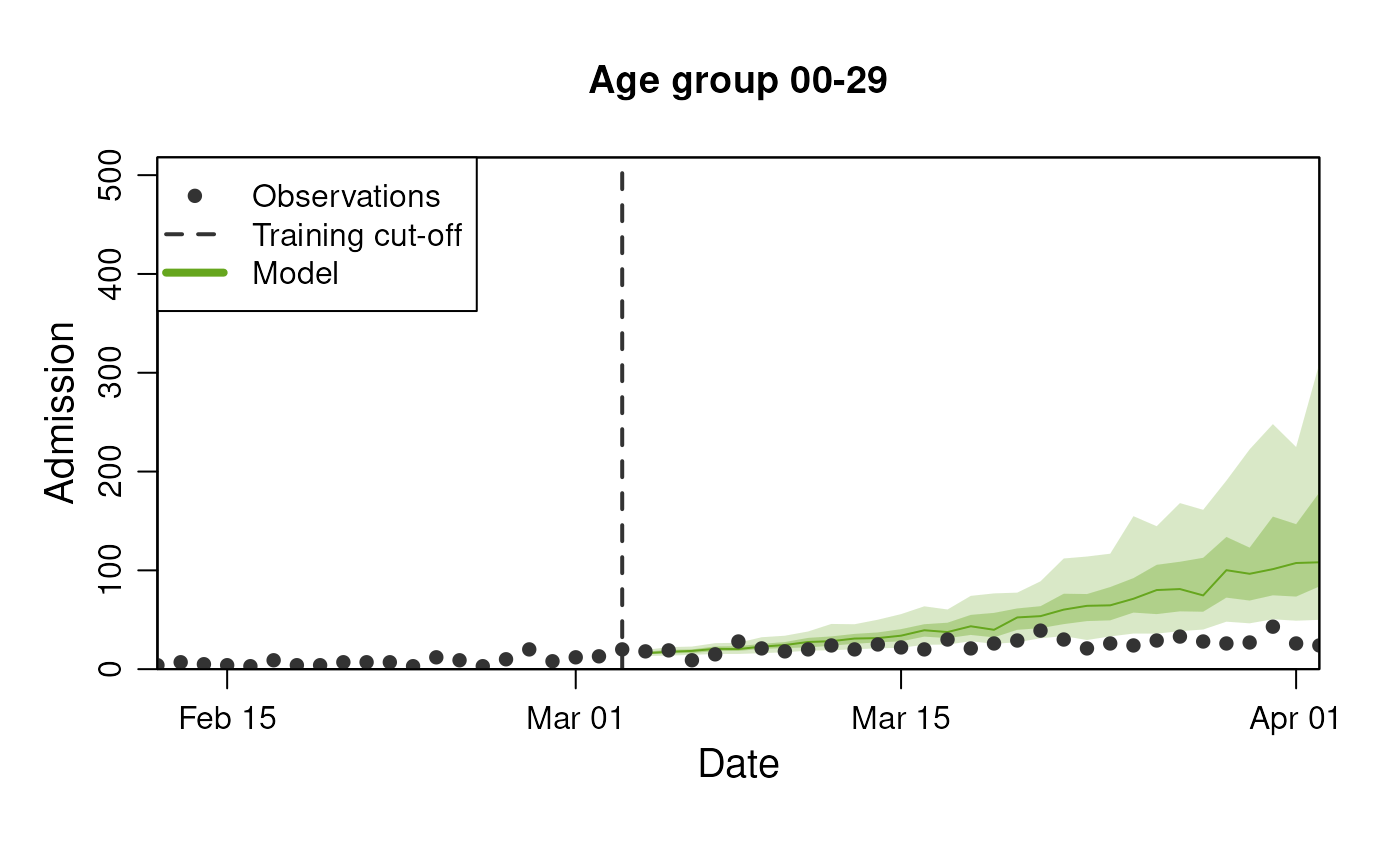
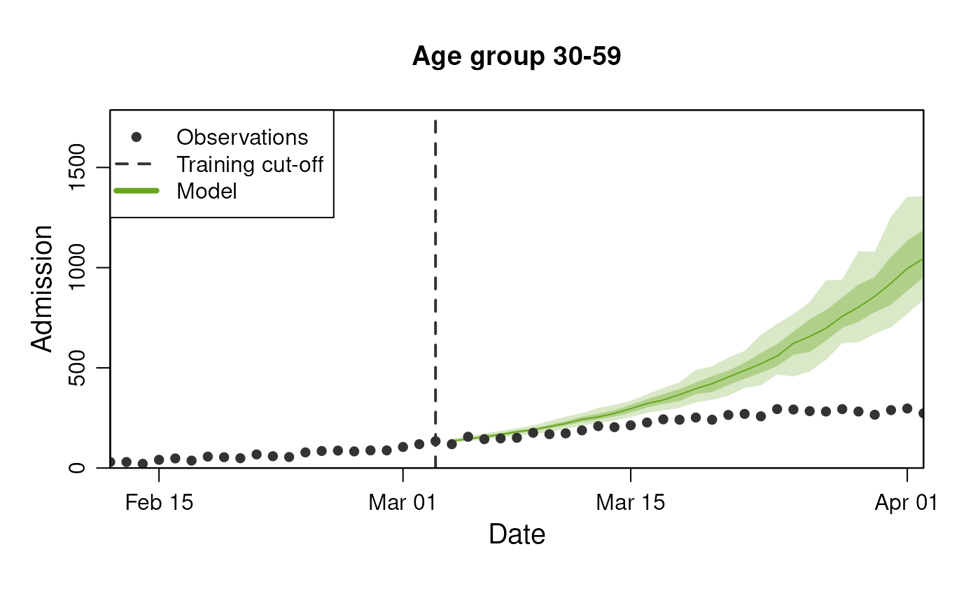
• n_admissions: The number of new hospital admissions due to infections (risk of hospitalisation dependent on age group).

When running the models, we should also define at what point in time they should provide predictions for. This is done by setting the last_queryable_date in the observables module:

last_queryable_date <- observables$ds$min_start_date + 60

Lets first look at the data we have available:

observables$get_observation(
  observable = "n_positive",
  stratification = rlang::quos(age_group),
  start_date = observables$ds$min_start_date,
  end_date = observables$ds$max_end_date
) |>
  ggplot2::ggplot(ggplot2::aes(x = date, y = n_positive)) +
  ggplot2::geom_vline(
    xintercept = last_queryable_date,
    color = "black",
    linetype = "dashed"
  ) +
  ggplot2::geom_point(color = "seagreen") +
  ggplot2::labs(title = "Observed number of positive cases") +
  ggplot2::facet_grid(~ age_group)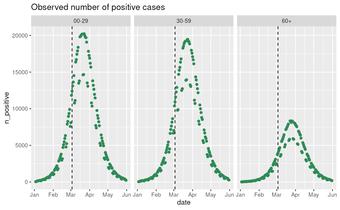

observables$get_observation(
  observable = "n_admission",
  stratification = rlang::quos(age_group),
  start_date = observables$ds$min_start_date,
  end_date = observables$ds$max_end_date
) |>
  ggplot2::ggplot(ggplot2::aes(x = date, y = n_admission)) +
  ggplot2::geom_vline(
    xintercept = last_queryable_date,
    color = "black",
    linetype = "dashed"
  ) +
  ggplot2::geom_point(color = "violetred3") +
  ggplot2::labs(title = "Number of admissions") +
  ggplot2::facet_grid(~ age_group)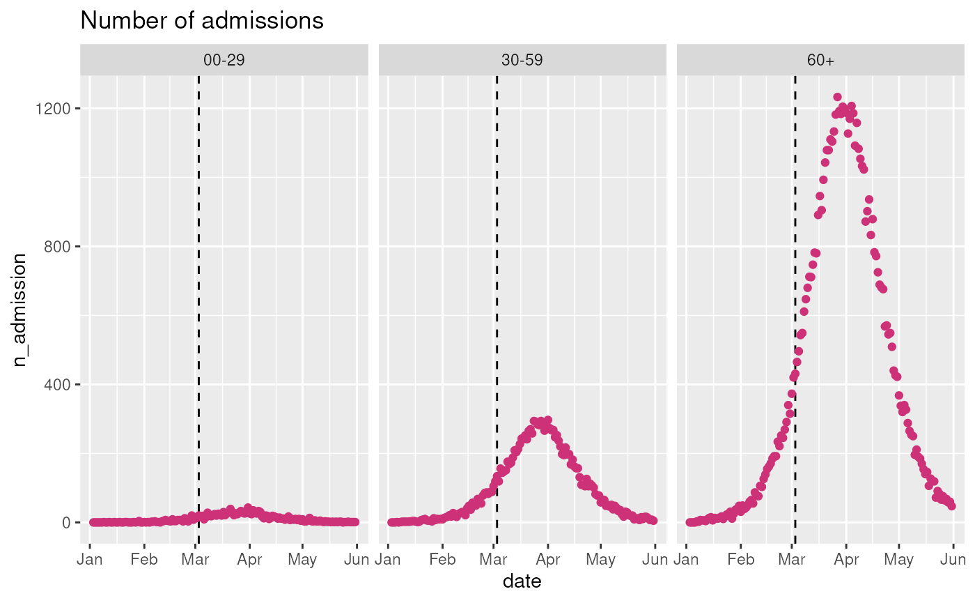

Applying the models to the data

The regressions models are special class of models which can directly model the data, and requires essentially no configuration.

Since the models are “duplicated” as described above, we here show only the results for the GLM family of models

observables$set_last_queryable_date(last_queryable_date)
model_1 <- DiseasyModelG0$new(observables = observables)
model_2 <- DiseasyModelG1$new(observables = observables)

The models are configured out-of-the-box and we can now retrieve model predictions for any observable:

model_1$get_results(
  observable = "n_positive",
  prediction_length = 30
)
#> # A tibble: 3,000 × 4
#>    date       n_positive realisation_id weight
#>    <date>          <dbl> <chr>           <dbl>
#>  1 2020-03-04     23274. 1                   1
#>  2 2020-03-05     20767. 1                   1
#>  3 2020-03-06     23386. 1                   1
#>  4 2020-03-07     23290. 1                   1
#>  5 2020-03-08     21900. 1                   1
#>  6 2020-03-09     19036. 1                   1
#>  7 2020-03-10     19889. 1                   1
#>  8 2020-03-11     20814. 1                   1
#>  9 2020-03-12     21250. 1                   1
#> 10 2020-03-13     25260. 1                   1
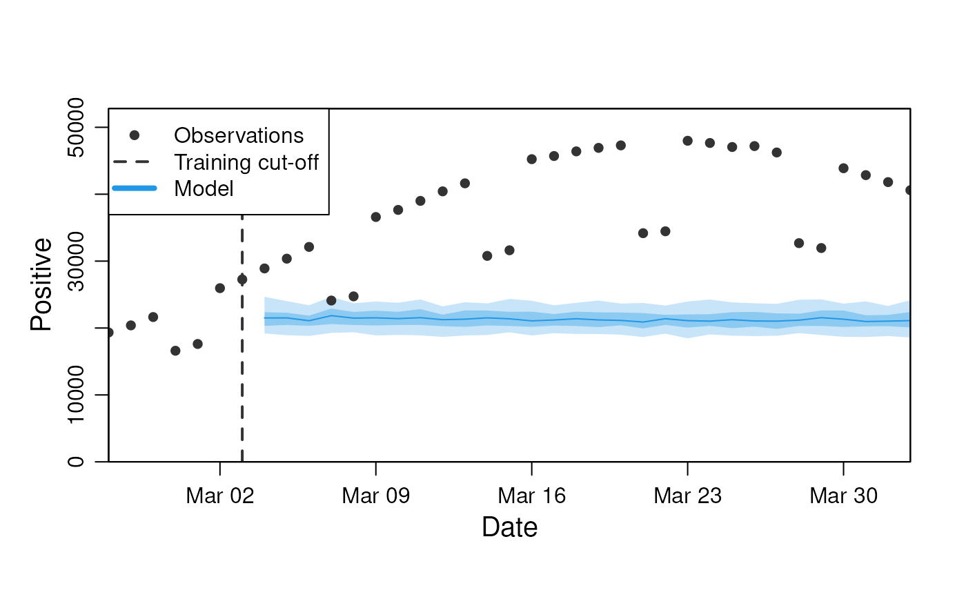
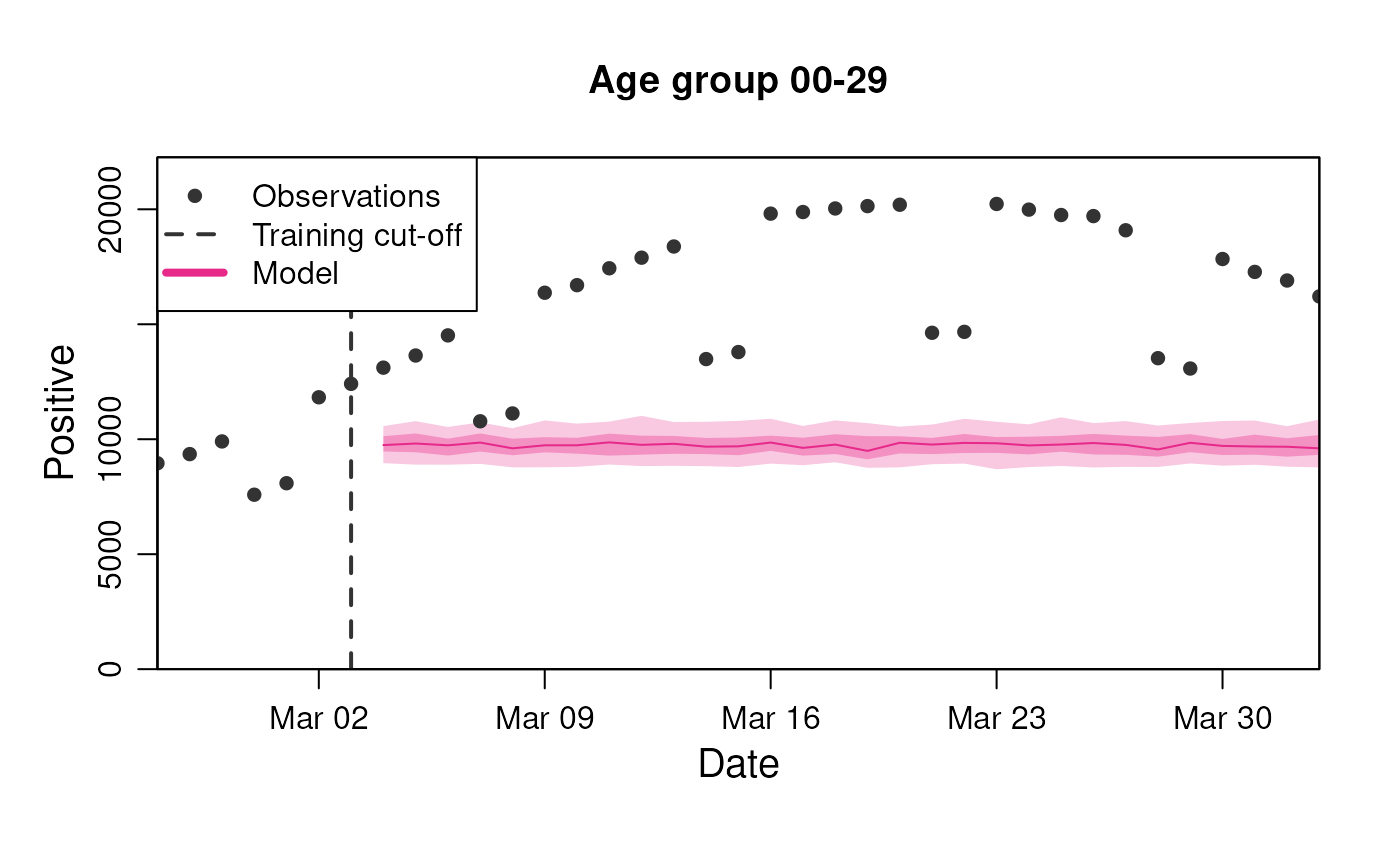
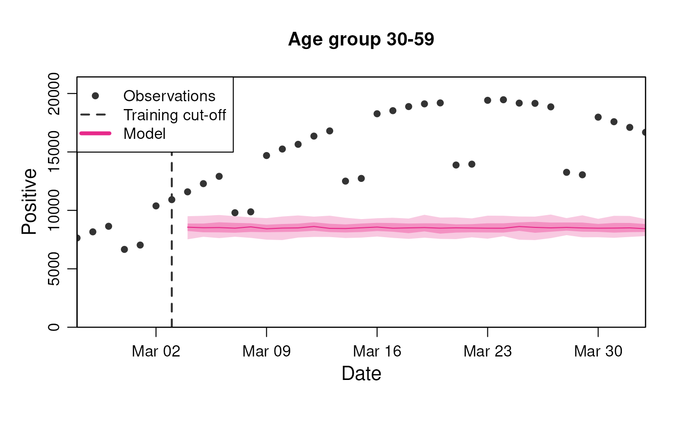
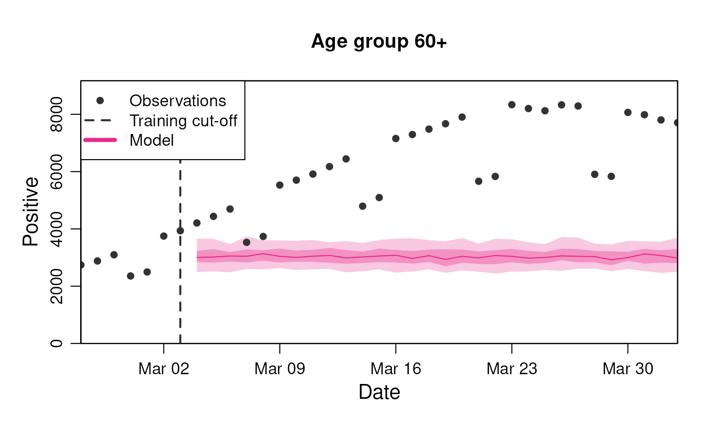
#> # ℹ 2,990 more rows

To visualise these predictions, we can use the standard plot() method where we supply the observable to predict and the number of days to predict into the future, as well as any stratification supported by the diseasystore.

Example plots for the constant predictor model

plot(
  model_1,
  observable = "n_positive",
  prediction_length = 30
)

plot(
  model_1,
  observable = "n_positive",
  stratification = rlang::quos(age_group),
  prediction_length = 30
)

Example plots for the exponential growth predictor model

plot(
  model_2,
  observable = "n_admission",
  prediction_length = 30
)

plot(
  model_2,
  observable = "n_admission",
  stratification = rlang::quos(age_group),
  prediction_length = 30
)