SEIR: Implementation

Introduction

This vignette is a companion to the implementation of the SEIR ode model ?DiseasyModelOdeSEIR.

As the name suggests, this model is a SEIR-like ordinary differential equation (ODE) model. Furthermore, the model is designed as flexible as possible to allow for a wide range of different model configuration. That is, the number of consecutive exposed, infected, and recovered states can be set arbitrarily, as well as the number of age groups and the number of variants.

Due to the flexibility of the model, the implementation is somewhat complex, which is why we include this vignette outlining the mathematical implementation of the model and connect it to the code.

Opening consideration

The design of the SEIR model is meant to be “standard” in the sense that it, in general, follows the structure and design of SEIR models in the community.

For clarity, we here describe the considerations needed to design the model.

Indexes and accents

To begin, here we define a fixed meaning to the different indices and accents used in the vignette:

Symbol	Description
$K,k$	Exposed states
$L,l$	Infected states
$M,m$	Recovered states
$A,i,j$	Age groups
$V,a,b$	Variants
$^\sim$	Non-normalised quantity

Where upper case letters denote the number of such elements and lower case letters denote a specific element.

The model structure

The SEIR model we are building is a compartmental model with (near) arbitrary number of exposed, infected, and recovered compartments. The model also supports multiple age groups and multiple variants.

We divide the model into different “tracks” with each track implementing the disease progression for a group of individuals. That is, if we have $A$ age groups and $V$ variants, we have $A \cdot V$ tracks which each start with the first exposed state (or the first infected state if no exposed states are included in the model). As the infection progresses within each individual, they are moved down the track through infection and eventually into recovery.

Schematically, the model can be represented as in the figure below:

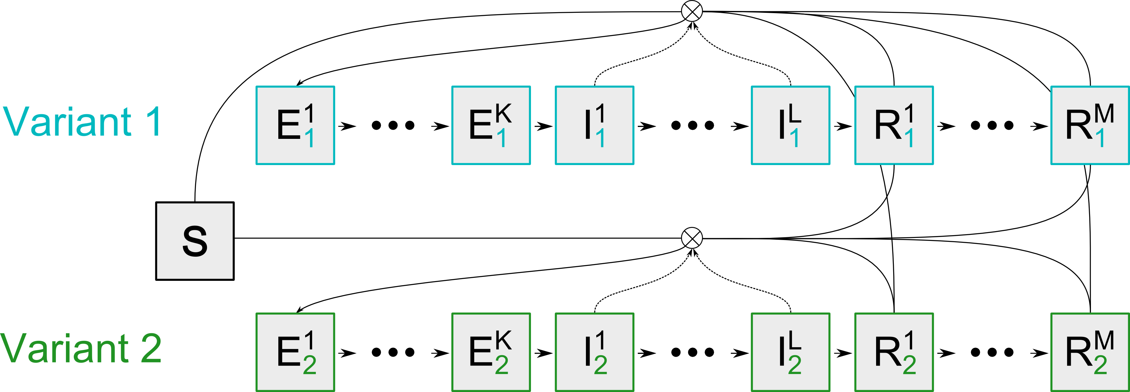
SEIR model overview for a two variant model

This figure shows the disease progression for two variant tracks for a single age group. The arrows in the figure indicates the infections in the model within these tracks.

State vector

Each “track” of infection is placed in sequence in the state vector, $\overline{\psi}$, and increments first in age groups then in variants.

Finally, the susceptible states are placed at the end of the state vector.

$$\overline{\psi} = [\underbrace{\begin{matrix} E_{1,1}^1\, \cdots \, E_{1,1}^K \;\;\; I_{1,1}^1 \, \cdots \, I_{1,1}^L \;\;\; R_{1,1}^1 \, \cdots \, R_{1,1}^M \end{matrix}}_{\text{Age group 1, Variant 1}}$$$$\underbrace{\begin{matrix} E_{2,1}^1 \, \cdots \, E_{2,1}^K \;\;\; I_{2,1}^1 \, \cdots \, I_{2,1}^L \;\;\; R_{2,1}^1 \, \cdots \, R_{2,1}^M \end{matrix}}_{\text{Age group 2, Variant 1}} \; \cdots$$$$\underbrace{\begin{matrix} E_{A,V}^1 \, \cdots \, E_{A,V}^K \;\;\; I_{A,V}^1 \, \cdots \, I_{A,V}^L \;\;\; R_{A,V}^1 \, \cdots \, R_{A,V}^M \end{matrix}}_{\text{Age group A, Variant V}} \;\; S_1 \, \cdots \, S_A]$$ NOTE: State vector uses normalised (unit) populations.

Notice that the state vector elements are indexed by state-type, state-index, age-index and variant-index:

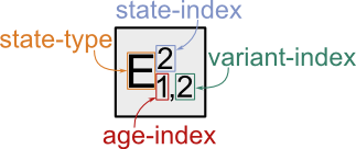
Index guide for the state vector

Contact matrix

The contact matrix, $\tilde{\overline{\overline{C}}}$, is a $A \times A$ matrix. The elements $\tilde{c}_{ij}$ can denotes the contacts from age group $j$ to age group $i$. (It may be helpful to memorise as $\tilde{c}_{i\leftarrow j}$)

In the model, these are normalised to the “per capita” contact matrix $\overline{\overline{C}}$, meaning that the elements are $c_{ij} = \frac{\tilde{c}_{ij}}{N_j}$ where $\tilde{N}_i$ is the population of age group $i$.

This way, when used in the model, the equations’ infections terms becomes: $\frac{\tilde{c}_{ij}}{\tilde{N}_j} \sum_l I_j^l S_i$ and the equations can be normalised via the transformations $\psi^e = \frac{\tilde{\psi}^e_{i|e}}{\tilde{N}_{i}}$, where $i|e$ is the age group of element $e$.

NOTE: Shouldn’t we then have $c_{ij} = \tilde{c}_{ij} \tilde{N}_j$ instead?

$$\dot{\tilde{I}} = \tilde{\beta}\, \tilde{I} \tilde{S} - r_I \tilde{I} \Rightarrow$$$$\frac{\dot{\tilde{I}}}{N} = \frac{\tilde{\beta}\, \tilde{I} \tilde{S}}{N} - \frac{ r_I \tilde{I}}{N} \Rightarrow$$$$\dot{I} = \tilde{\beta}\, I \tilde{S} - r_I I \Rightarrow$$

$$\dot{I} = N\tilde{\beta}\, I \frac{\tilde{S}}{N} - r_I I \Rightarrow$$

$$\dot{I} = \underbrace{N\tilde{\beta}}_{\beta}\, I S - r_I I$$

The implementation of the right-hand side function

With the opening considerations in mind, we can now describe the implementation of the model. Below, we now link the implementation with the underlying mathematical descriptions of the model.

The ?DiseasyModelOdeSEIR model implements the $rhs method which computes the rates needed for the ODE solver. The evaluation of this right-hand side function uses a few intermediate variables which are described below.

The infected matrix

In the computation of the right-hand side of the ODE, we have a helper matrix $\overline{\overline{I}}$ stored as infected in the implementation.

This $\overline{\overline{I}}$ matrix is a $A \times V$ matrix with elements

$$\overline{\overline{I}} = \begin{bmatrix} \sum_l I^l_{1,1} & \cdots & \sum_l I^l_{1,V} \\ \vdots & \ddots & \vdots \\ \sum_l I^l_{A,1} & \cdots & \sum_l I^l_{A,V} \end{bmatrix}$$

That is, the element $i_{a, v}$ contains the sum of all infected compartments for the track associated with age group $a$ and variant $v$.

The infected_contact_rate matrix

During the right-hand side computation, we also have a helper matrix infected_contact_rate which is $\overline{\overline{C}}\; \overline{\overline{I}}$

$$\overline{\overline{CI}} = \overline{\overline{C}}\; \overline{\overline{I}} = \begin{bmatrix} \sum_i c_{1\leftarrow i} \sum_l I^l_{i,1} & \cdots & \sum_i c_{1\leftarrow i} \sum_l I^l_{i,V} \\ \vdots & \ddots & \vdots \\ \sum_i c_{A\leftarrow i} \sum_l I^l_{i,1} & \cdots & \sum_i c_{A\leftarrow i} \sum_l I^l_{i,V} \end{bmatrix}$$

That is, the element $(\overline{\overline{CI}})_{i, a}$ contains the rate of contact for age group $i$ with persons infected with variant $a$ across all age groups.

The infection_rate matrix

Continuing the computation of the right-hand side, we have the infection_rate matrix ($\overline{\overline{T}}$) which is the infected_contact_rate ($\overline{\overline{CI}}$) adjusted for additional risk factors.

• $\sigma(t)$: Multiplicative effect of season
• $\epsilon_a$: Relative infectiousness of variant $a$
• $\Gamma$: Overall infection rate scaling factor

$$\overline{\overline{T}} = \Gamma\;\sigma(t)\;\overline{\overline{\mathcal{E}}} \odot \overline{\overline{CI}}$$

Where $\odot$ is the Hadamard product (element-wise multiplication), and $\overline{\overline{\mathcal{E}}}$ is the $A \times V$ matrix:

$$\overline{\overline{\mathcal{E}}} = \begin{bmatrix} \epsilon_1 & \cdots & \epsilon_V \\ \vdots & \ddots & \vdots \\ \epsilon_1 & \cdots & \epsilon_V \end{bmatrix}$$

NOTE: In the code, private$indexed_variant_infection_risk is $\overline{\overline{\mathcal{E}}}$ in vector form.

The infection_matrix

For the final computation of infections of the right-hand side, we construct the matrix infection_matrix ($\overline{\overline{f}}$).

Since only $R$ and $S$ compartments are susceptible to infection, we need only to consider the $RS$ states to compute the new infections in the model.

The new infection_matrix therefore does not need to contain the K exposed states and the L infected states, but only the M recovered states and the $A$ susceptible states.

We are therefore interested in the reduced state vector $\overline{\psi}^{RS}$ whose elements $e^*$ are the $R$ and $S$ elements of the full state vector $\overline{\psi}$.

We now create an intermediate matrix $\overline{\overline{U}}$ by expanding the infection_rate matrix ($\overline{\overline{T}}$) to a $A \cdot (V \cdot M + 1) \times V$ matrix by repeating the rows of the infection_rate matrix. This repeating is done by matching the age group of the infection_rate matrix to the age group of the reduced state vector. Each element, $e$, in the state vector, $\psi$ has a corresponding age group which we can write as $i|e$.

The intermediate matrix $\overline{\overline{U}}$, has a row for all states in $R$ or $S$ compartments and column for each variant. The form is as follows:

$$\overline{\overline{U}} = \begin{bmatrix} t_{i|e^*_1, 1} & \cdots & t_{i|e^*_1, V} \\ t_{i|e^*_2, 1} & \cdots & t_{i|e^*_2, V} \\ \vdots & \vdots &\vdots \\ t_{i|e^*_{A \cdot (V \cdot M + 1)}, 1} & \cdots & t_{i|e^*_{A \cdot (V \cdot M + 1)}, V} \\ \end{bmatrix}$$

We now have a matrix, whose elements are the infection rate for each variant matched to the $R$ and $S$ elements of the state vector.

In this space, we can now account for:

• The state specific infection risks (i.e. the reduced risk from being infected previously / vaccinated)
• The effect of cross-immunity between the variants

That is, we need to construct the matrix that accounts for the waning of immunity ($\gamma_m$) and the cross-immunity factors $\chi_{a\leftarrow b}$ (Variant $b$ infecting a person with immunity for variant $a$).

All together, this is implemented via the immunity matrix (immunity_matrix) $\overline{\overline{\rho}}$ which is $A \cdot (V \cdot M + 1) \times V$ matrix on the form:

$$\overline{\overline{\rho}} = \begin{bmatrix} \begin{bmatrix} 1 - \chi_{1\leftarrow 1} (1 - \overline{\gamma}) \\ \vdots \\ 1 - \chi_{1\leftarrow 1} (1 - \overline{\gamma}) \end{bmatrix} & \cdots & \begin{bmatrix} 1 - \chi_{1\leftarrow V} (1 - \overline{\gamma}) \\ \vdots \\ 1 - \chi_{1\leftarrow V} (1 - \overline{\gamma}) \end{bmatrix} \\ \vdots & \ddots & \vdots \\ \begin{bmatrix} 1 - \chi_{V\leftarrow 1} (1 - \overline{\gamma}) \\ \vdots \\ 1 - \chi_{V\leftarrow 1} (1 - \overline{\gamma}) \end{bmatrix} & \cdots & \begin{bmatrix} 1 - \chi_{V\leftarrow V} (1 - \overline{\gamma}) \\ \vdots \\ 1 - \chi_{V\leftarrow V} (1 - \overline{\gamma}) \end{bmatrix} \\ \overline{1}_A & \cdots & \overline{1}_A \end{bmatrix}$$

Where $\overline{1}_A$ is a ones vector of length $A$.

In $\overline{\overline{\rho}}$, the sub-matrices of the form:

$$\begin{bmatrix} 1 - \chi_{a\leftarrow b} (1 - \overline{\gamma}) \\ \vdots \\ 1 - \chi_{a\leftarrow b} (1 - \overline{\gamma}) \end{bmatrix}$$

are $A \cdot M \times 1$ matrices with repeated sub-matrices. That is, $1 - \chi_{a\leftarrow b} (1 - \overline{\gamma})$ is a vector of length $M$ which is repeated for each age group, to form the $A \cdot M \times 1$ matrix.

In total, the matrix accounts for the cross-variant $\chi_{a\leftarrow b}$ reductions of immunity ($1-\overline{\gamma}$).

Finally, we can combine everything to the flow matrix:

$$\overline{\overline{f}} = \overline{\overline{\rho}} \odot \begin{bmatrix} \vert & & \vert \\ \overline{\psi}^{RS} & \cdots & \overline{\psi}^{RS} \\ \vert & & \vert \\ \end{bmatrix} \odot \overline{\overline{U}}$$

Where $\begin{bmatrix}\overline{\psi}^{RS} & \cdots & \overline{\psi}^{RS}\end{bmatrix}$ is $V$ repeats of the $R$ and $S$ elements of the state vector $\overline{\psi}$.

This matrix contains, for each $R$ and $S$ element in the state vector, a row consisting of per-variant infectious contacts between the corresponding compartment and the infected population in the model. These elements account for every risk modifying mechanism included in the model.

The row sums of this matrix is then equal to the loss from the compartment due to infectious contacts. The sums by variant/age group combination can also be extracted from the matrix to form the in-flow of new infections to the $E_1$ compartments.

Generator matrix

Beyond implementing the right-hand side of the ODE, we also implement the generator matrix for the model.

The generator matrix, $\overline{\overline{G}}$, is a $A \cdot V \cdot (K+L) \times A \cdot V \cdot (K+L)$ matrix containing the dynamics of the $E$ and $I$ states under the assumption of static $R$ and $S$ states.

Formally, the generator matrix is the linearisation:

$$\frac{d\overline{\psi}^{EI}}{d t} = \overline{\overline{G}} \overline{\psi}^{EI}$$

The matrix can be decomposed into two contributions:

• The transition matrix, $\overline{\overline{G}}_T$, which is a bi-diagonal matrix containing the flow rates between sequential compartments
• The transmission matrix, $\overline{\overline{G}}_\beta$ which contains the flows stemming from infections.

The transition matrix is block-diagonal and has the form (here for $K = 1$ and $L = 1$ and $A + V > 2)$:

$$\overline{\overline{G}}_T = \left[\begin{array}{cccc} \begin{bmatrix} -r_e & 0 \\ r_e & -r_i \end{bmatrix} & \begin{matrix} 0 & 0 \\ 0 & 0 \end{matrix} & \cdots & \begin{matrix} 0 & 0 \\ 0 & 0 \end{matrix} \\ \begin{matrix} 0 & 0 \\ 0 & 0 \end{matrix} & \begin{bmatrix} -r_e & 0 \\ r_e & -r_i \end{bmatrix} & \cdots & \begin{matrix} 0 & 0 \\ 0 & 0 \end{matrix} \\ \vdots & \vdots & \ddots & \vdots \\ \begin{matrix} 0 & 0 \\ 0 & 0 \end{matrix} & \begin{matrix} 0 & 0 \\ 0 & 0 \end{matrix} & \cdots & \begin{bmatrix} -r_e & 0 \\ r_e & -r_i \end{bmatrix} \end{array}\right]$$

Notice that the off-diagonal has zero-elements where the (reduced) state vector changes age groups ($I_i^L \rightarrow E_{i+1}^1$).

The form of the transmission matrix is more difficult to write up.

We lump risk modifying factors such as the effect of season $\sigma(t)$ and overall infection rate $\Gamma$ into a single factor $\beta$.

Some examples:

Double age group, single variant

As long as we have only a single variant, cross immunity can be ignored and we can lump the effect of the balance between $R$ to $S$ into $\beta$.

For $K = 1$ and $L = 1$, the transmission matrix is:

$$\overline{\overline{G}}_\beta = \beta \begin{bmatrix} 0 & c_{1\leftarrow 1} & 0 & c_{1\leftarrow 2} \\ 0 & 0 & 0 & 0 \\ 0 & c_{2\leftarrow 1} & 0 & c_{2\leftarrow 2} \\ 0 & 0 & 0 & 0 \end{bmatrix}$$

For $K = 1$ and $L = 2$, the transmission matrix is:

$$\overline{\overline{G}}_\beta = \beta \begin{bmatrix} 0 & c_{1\leftarrow 1} & c_{1\leftarrow 1} & 0 & c_{1\leftarrow 2} & c_{1\leftarrow 2} \\ 0 & 0 & 0 & 0 & 0 & 0\\ 0 & 0 & 0 & 0 & 0 & 0\\ 0 & c_{2\leftarrow 1} & c_{2\leftarrow 1} & 0 & c_{2\leftarrow 2} & c_{2\leftarrow 2} \\ 0 & 0 & 0 & 0 & 0 & 0\\ 0 & 0 & 0 & 0 & 0 & 0 \end{bmatrix}$$

Single age group, double variant

With only one age group, the contact matrix is the scalar $c$.

With two variants, we need to also account for the relative infectivity of the variants $\epsilon_a$.

Then, for $K = 1$ and $L = 1$, the transmission matrix is:

$$\overline{\overline{G}}_\beta = \beta\left[ \begin{array}{ccccc} 0 & \epsilon_1\hat{\rho}_{1}\,c & | & 0 & 0 \\ 0 & 0 & | & 0 & 0 \\ - & - & + & - & - \\ 0 & 0 & | & 0 & \epsilon_2\hat{\rho}_{2}\,c \\ 0 & 0 & | & 0 & 0 \end{array} \right]$$

Where the change between variants is demarcated visually by the vertical and horizontal lines. We now have the additional factor $\hat{\rho}$ which explicitly accounts for the balance of $S$ and $R$ states and the cross-immunity between the variants:

$$\hat{\rho}_{a} = S + \sum_{b = 1}^V\sum_{m=1}^M \left(1 - \chi_{b \leftarrow a}(1 - \gamma_m)\right) R^m_b$$

That is, we have the unmodified contribution from the $S$ states, and the contribution from all $R$ states while accounting for waning of immunity ($\gamma_m$) and cross-immunity ($\chi_{a \leftarrow b}$).

This factor is analogous to a “cross-section” of infection encounter, i.e. a factor that accounts for the probability that a contact between an infectious and non-infected person is an infectious contact.

Then, for $K = 1$ and $L = 2$, the transmission matrix is:

$$\overline{\overline{G}}_\beta = \beta\left[ \begin{array}{ccccccc} 0 & \epsilon_1\hat{\rho}_{1}\,c & \epsilon_1\hat{\rho}_{1}\,c & | & 0 & 0 & 0 \\ 0 & 0 & 0 & | & 0 & 0 & 0 \\ 0 & 0 & 0 & | & 0 & 0 & 0 \\ - & - & - & + & - & - & - \\ 0 & 0 & 0 & | & 0 & \epsilon_2\hat{\rho}_{2}\,c & \epsilon_2\hat{\rho}_{2}\,c \\ 0 & 0 & 0 & | & 0 & 0 & 0 \\ 0 & 0 & 0 & | & 0 & 0 & 0 \\ \end{array} \right]$$

Double age group, double variant

When including age groups, the $\hat{\rho}$ factor becomes a $A \times V$ matrix of elements

$$\hat{\rho}_{i, a} = S_i + \sum_{b = 1}^V\sum_{m=1}^M \left(1 - \chi_{b \leftarrow a}(1 - \gamma_m)\right) R^m_{i,b}$$

For $K = 1$ and $L = 1$, the transmission matrix is:

$$\overline{\overline{G}}_\beta = \beta\left[ \begin{array}{cccccccc} 0 & \epsilon_1\hat{\rho}_{1,1}\,c_{1\leftarrow 1} & 0 & \epsilon_1\hat{\rho}_{1,1}\,c_{1\leftarrow 2} & | & 0 & 0 & 0 & 0 \\ 0 & 0 & 0 & 0 & | & 0 & 0 & 0 & 0\\ 0 & \epsilon_1\hat{\rho}_{2,1}\,c_{2\leftarrow 1} & 0 & \epsilon_1\hat{\rho}_{2,1}\,c_{2\leftarrow 2} & | & 0 & 0 & 0 & 0 \\ 0 & 0 & 0 & 0 & | & 0 & 0 & 0 & 0 \\ - & - & - & - & + & - & - & - & - \\ 0 & 0 & 0 & 0 & | & 0 & \epsilon_2\hat{\rho}_{1,2}\,c_{1\leftarrow 1} & 0 & \epsilon_2\hat{\rho}_{1,2}\,c_{1\leftarrow 2} \\ 0 & 0 & 0 & 0 & | & 0 & 0 & 0 & 0 \\ 0 & 0 & 0 & 0 & | & 0 & \epsilon_2\hat{\rho}_{2,2}\,c_{2\leftarrow 1} & 0 & \epsilon_2\hat{\rho}_{2,2}\,c_{2\leftarrow 2} \\ 0 & 0 & 0 & 0 & | & 0 & 0 & 0 & 0 \end{array} \right]$$

Notes on optimisations of the right-hand side function

It is important that the implementation is somewhat optimised for the simulations to run in reasonable time. To that end, we here show micro-benchmarks of different implementations of the same steps to highlight why a given implementation was chosen.

These benchmarks assume a simple SEIR model with only tree age group and one variant.

“infected” sum computation

## Step 1, determine the number of infected by age group and variant
i_state_indices <- list(2, 5, 8)
state_vector <- rep(0, 9)

# Benchmark possible approaches
microbenchmark::microbenchmark( # Microseconds
  "purrr::map_dbl" = purrr::map_dbl(
    i_state_indices,
    \(indices) sum(state_vector[indices])
  ),
  "sapply" = sapply(
    i_state_indices,
    \(indices) sum(state_vector[indices])
  ),
  "sapply - USE.NAMES" = sapply(
    i_state_indices,
    \(indices) sum(state_vector[indices]),
    USE.NAMES = FALSE
  ),
  "vapply" = vapply(
    i_state_indices,
    \(indices) sum(state_vector[indices]),
    FUN.VALUE = numeric(1),
    USE.NAMES = FALSE
  ),
  check = "equal", times = 1000L
)
#> Unit: microseconds
#>                expr    min     lq      mean  median      uq      max neval
#>      purrr::map_dbl 25.347 27.822 31.539710 28.9040 30.0010 2045.024  1000
#>              sapply 12.815 13.445 14.452131 13.9010 14.8630   32.501  1000
#>  sapply - USE.NAMES 12.894 13.445 14.350858 13.8455 14.7280   38.723  1000
#>              vapply  4.869  5.370  5.725077  5.6310  5.8305   33.492  1000