SEIR: Accounting for structural differences in malthusian growth rates

library(diseasy)
#> Loading required package: diseasystore
#> 
#> Attaching package: 'diseasy'
#> The following object is masked from 'package:diseasystore':
#> 
#>     diseasyoption

Introduction

When using a generalised SEIR model with $K$ and $L$ consecutive $E$ and $I$ states respectively, there are some structural differences in the realised (Malthusian) growth rate of the system for the same contact rate $\beta$.

Since we would like to be able to compare different SEIR models with different compartment structures, we would like to be able to account for this difference in scaling of the growth rates.

Following the method outlined by Diekmann et al., we compute the Malthusian growth rate in the system and scale the contact rates such that the system achieves the same Malthusian growth rate as a SIR model with the same contact rate $\beta$.

Visualisation

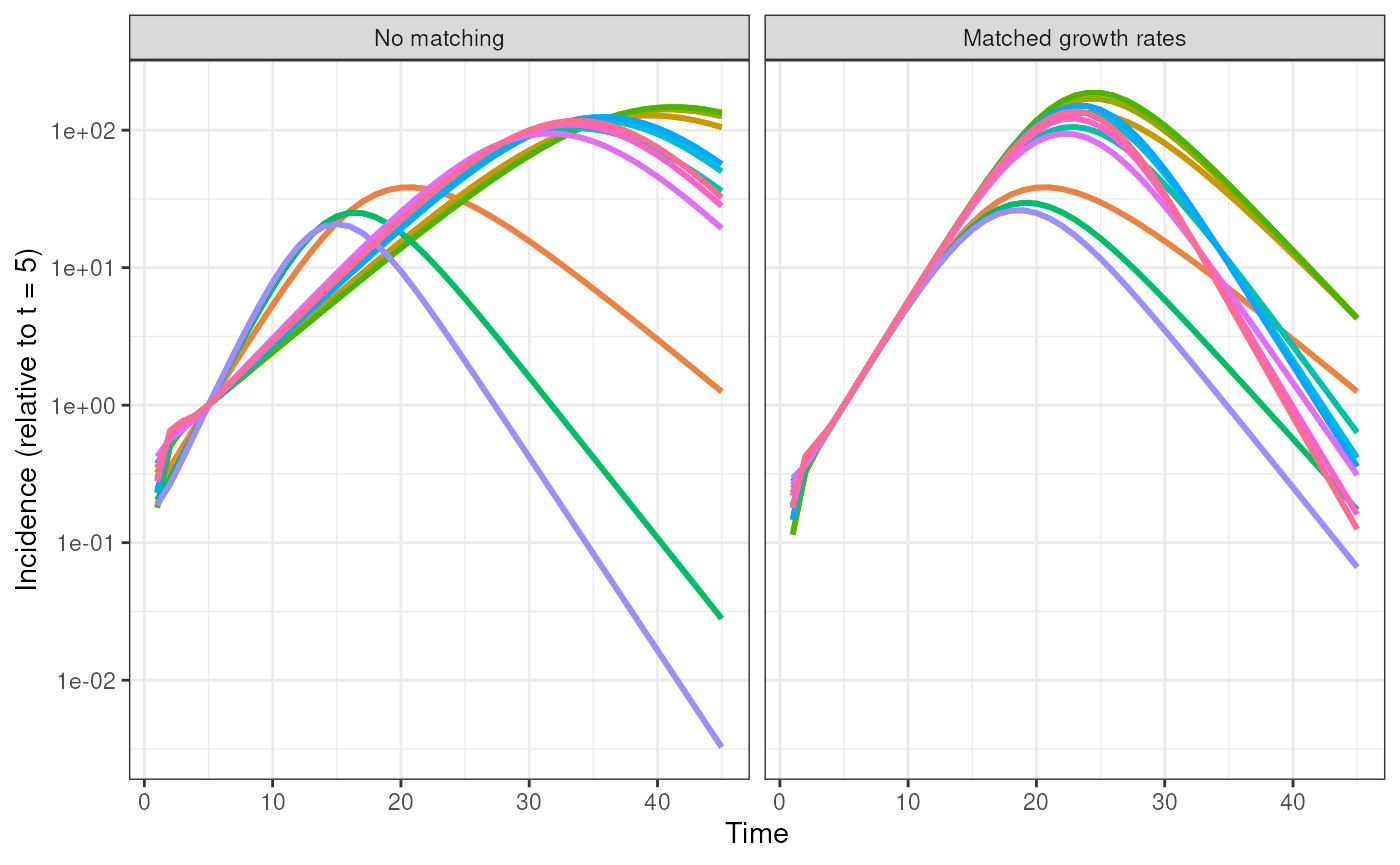
Below we run all SEIR models with 0-3 $E$ and 1-3 $I$ states with and without age groups all using the same contact rate $\beta$, and compare the incidence from the models over time.

These models are run both with and without the Malthusian growth rate matching.

Notice that the when the Malthusian growth rates are matched, the matching is done to the SIR model which has faster growth than the SEIR model with the same contact rate $\beta$.

# Set the time scales of the problem
rE <- 1 / 2
rI <- 1 / 4

tmax <- 45

# Set the combinations to test
combinations <- tidyr::expand_grid(
  K = seq.int(0, 3),
  L = seq.int(3),
  age_cuts_lower = list(0, c(0, 30, 60))
)

combinations |>
  purrr::pmap(\(K, L, age_cuts_lower) {

    purrr::map(c(FALSE, TRUE), \(match) {
      # Run a SIR model to generate the target of our initialisation
      m <- DiseasyModelOdeSeir$new(
        observables = DiseasyObservables$new(
          conn = DBI::dbConnect(RSQLite::SQLite()),
          last_queryable_date = Sys.Date() - 1
        ),
        variant = DiseasyVariant$new(),
        parameters = list(
          "compartment_structure" = c("E" = K, "I" = L, "R" = 1L),
          "age_cuts_lower" = 0,
          "overall_infection_risk" = 0.6,
          "disease_progression_rates" = c("E" = rE, "I" = rI),
          "malthusian_matching" = match
        )
      )

      # Generate a uniform initial state_vector that sums to 1
      y0 <- c(rep(0, K + L + 1), 0.999)
      y0[1] <- 0.001

      # Run solver across scenario change to check for long-term leakage
      sol <- deSolve::ode(
        y = y0,
        times = seq(0, tmax),
        func = m %.% rhs,
        parms = NULL
      )

      # Retrieve the (incidence) signal
      data.frame(t = sol[, 1], incidence = L * rI * sol[, K + 2]) |>
        dplyr::mutate(
          incidence = incidence / incidence[6],
          model_configuration = glue::glue(
            "L = {L}, K = {K}, A = {length(age_cuts_lower)}"
          ),
          malthusian_matching = dplyr::if_else(
            condition = match,
            true = "Matched growth rates",
            false = "No matching"
          )
        ) |>
        dplyr::filter(t > 0)
    }) |>
      purrr::list_rbind()

  }) |>
  purrr::list_rbind() |>
  ggplot2::ggplot(ggplot2::aes(x = t, y = incidence, color = model_configuration)) +
    ggplot2::geom_line(linewidth = 1) +
    ggplot2::scale_y_continuous(transform = "log10") +
    ggplot2::facet_wrap(
      ~ factor(
        malthusian_matching,
        levels = c("No matching", "Matched growth rates")
      )
    ) +
    ggplot2::xlab("Time") +
    ggplot2::ylab("Incidence (relative to t = 5)") +
    ggplot2::guides(color = "none") +
    ggplot2::theme_bw()