DiseasyModelOde

library(diseasy)
#> Loading required package: diseasystore
#> 
#> Attaching package: 'diseasy'
#> The following object is masked from 'package:diseasystore':
#> 
#>     diseasyoption

Introduction

One of the model families in diseasy is the family of Ordinary Differential Equation (ODE) models. This family of models is presently represented only by the ?DiseasyModelOdeSeir, a model template that implements SEIR (Susceptible, Exposed, Infected, Recovered) ODE models according to user specification. This template allows for any number of $E$, $I$ or $R$ states in the model and interfaces with the ?DiseasySeason, ?DiseasyActivity, ?DiseasyVariant and ?DiseasyImmunity modules for scenario definitions.

The workflow for creating a specific ?DiseasyModelOdeSeir model would roughly follow these steps:

1. Defining the scenario. The first step to using most models in diseasy is to define the scenario. That is, to configure the functional modules that the model templates takes as argument (e.g. ?DiseasyActivity). These steps provide the model template with information about the population, the activity, variants to include etc.
2. Choosing the model configuration. The model template may have some configurability that you control. In the case of ?DiseasyModelOdeSeir for example, you must choose the number of consecutive $E$, $I$ and $R$ states in the model.
3. Mapping to observables. The ODE family of models is in some ways bespoke in the sense that the user needs provide a mapping from the observables to the “true” incidence of infections. The model is then initialised from this estimated incidence. If the model should provide predictions for observables other than the “true” incidence, the user needs to provide mapping between the model incidence and the observables in question.

These steps are outlined in individual sections below where we work through defining a model in a specific example. Note that this example is contrived in the sense that the data we use in this example have been generated with this exact model template and we therefore can match the observations near-perfectly.

Example data

The data we will use this example is provided by ?DiseasystoreSeirExample which represents data in a Danish context.

We first create an observables module to interface with this data:

# Configure a observables module with the example data and database
observables <- DiseasyObservables$new(
  diseasystore = DiseasystoreSeirExample,
  conn = DBI::dbConnect(RSQLite::SQLite())
)

The data is stratified by age and covers a single infection wave. It contains three observables of interest for our example:

• n_infected: The true number of infected in the data.
• n_positive: The observed subset of infected (65% of true infected are observed but fewer are observed during the weekend).
• n_admissions: The number of new hospital admissions due to infections (risk of hospitalisation dependent on age group).

When running the models, we should also define at what point in time they should provide predictions for. This is done by setting the last_queryable_date in the observables module:

last_queryable_date <- observables$ds$min_start_date + 40

Lets first look at the data we have available:

observables$get_observation(
  observable = "n_infected",
  stratification = rlang::quos(age_group),
  start_date = observables$ds$min_start_date,
  end_date = observables$ds$max_end_date
) |>
  ggplot2::ggplot(ggplot2::aes(x = date, y = n_infected)) +
  ggplot2::geom_vline(
    xintercept = last_queryable_date,
    color = "black",
    linetype = "dashed"
  ) +
  ggplot2::geom_point(color = "deepskyblue3") +
  ggplot2::labs(title = "True number of infected") +
  ggplot2::facet_grid(~ age_group)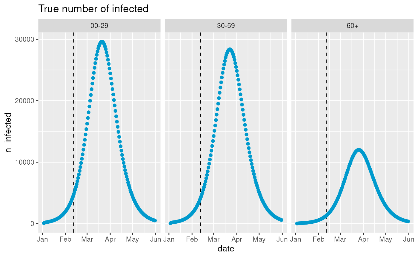

observables$get_observation(
  observable = "n_positive",
  stratification = rlang::quos(age_group),
  start_date = observables$ds$min_start_date,
  end_date = observables$ds$max_end_date
) |>
  ggplot2::ggplot(ggplot2::aes(x = date, y = n_positive)) +
  ggplot2::geom_vline(
    xintercept = last_queryable_date,
    color = "black",
    linetype = "dashed"
  ) +
  ggplot2::geom_point(color = "seagreen") +
  ggplot2::labs(title = "Observed number of positive cases") +
  ggplot2::facet_grid(~ age_group)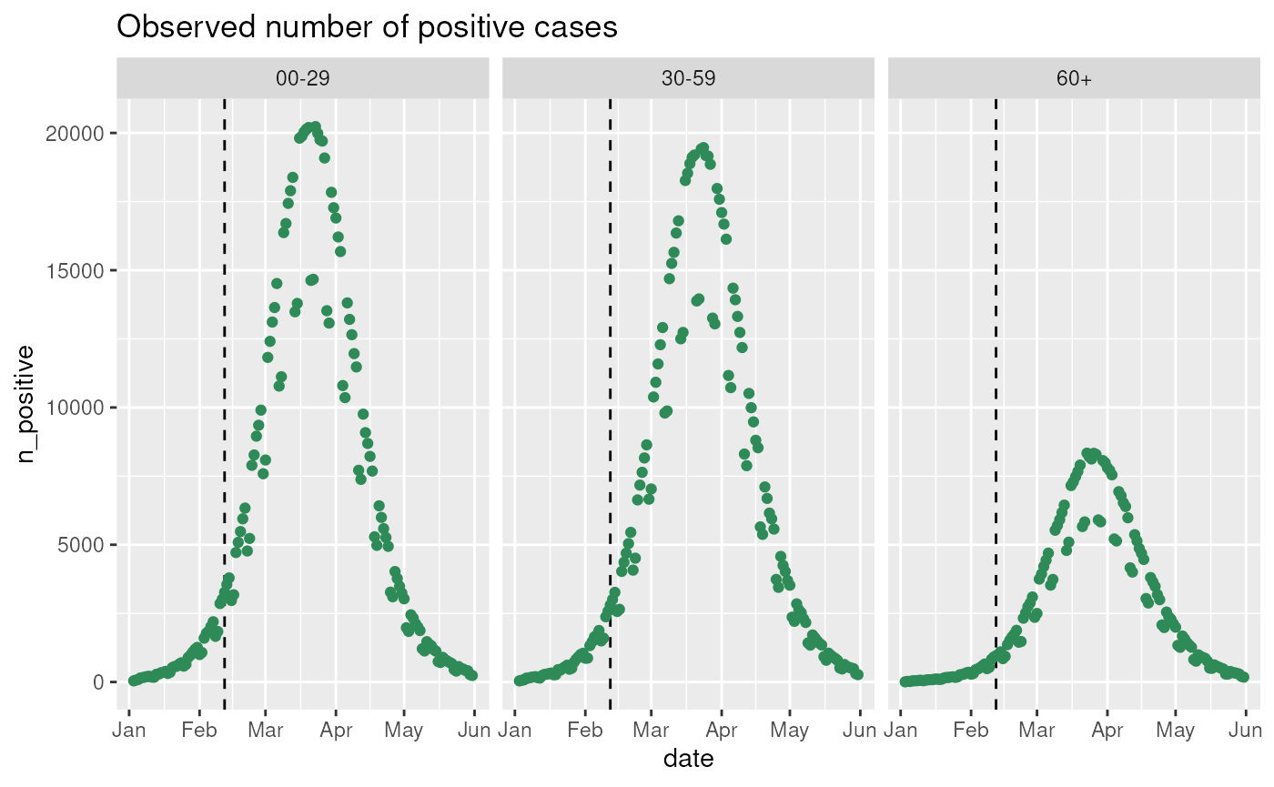

observables$get_observation(
  observable = "n_admission",
  stratification = rlang::quos(age_group),
  start_date = observables$ds$min_start_date,
  end_date = observables$ds$max_end_date
) |>
  ggplot2::ggplot(ggplot2::aes(x = date, y = n_admission)) +
  ggplot2::geom_vline(
    xintercept = last_queryable_date,
    color = "black",
    linetype = "dashed"
  ) +
  ggplot2::geom_point(color = "violetred3") +
  ggplot2::labs(title = "Number of admissions") +
  ggplot2::facet_grid(~ age_group)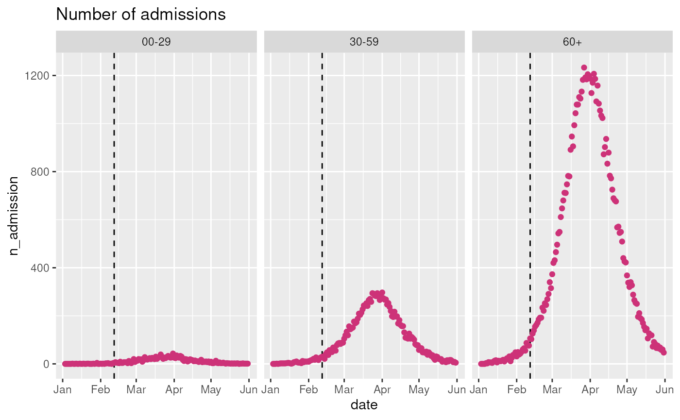

Defining the scenario

The first step to creating a ?DiseasyModelOdeSeir model is to define the scenario. In this case, as we stated above, we can exactly match the scenario to the data since the data was created using this class of models.

First we define the activity scenario via the ?DiseasyActivity module. This scenario describes the changes in activity in the society (e.g. restrictions). To see more on how to configure this module, see vignette("diseasy-activity").

# Configure an activity module using Danish population and contact information.
activity <- DiseasyActivity$new()
activity$set_contact_basis(contact_basis = contact_basis$DK)
activity$set_activity_units(dk_activity_units)

# The level of activity is fixed to the "baseline" level throughout the simulation.
activity$change_activity(date = as.Date("2020-01-01"), opening = "baseline")

This particular scenario does not include any more dynamics, but this would be the stage where the level of seasonality and the variant composition should be defined (see vignette("diseasy-season") and vignette("diseasy-variant") for more details).

Choosing the model configuration

The ?DiseasyModelOdeSeir model template has a number of hyperparameters and parameters that should be configured for the model to run.

The hyperparameters are:

• compartment_structure: A named vector specifying the number of consecutive $E$, $I$ and $R$ states in the model.
• age_cuts_lower: A vector of age cuts for the age groups in the model.

The parameters are:

• disease_progression_rates: A named vector specifying the progression rates from $E$ to $I$ and from $I$ to $R$ (i.e. waiting times).
• overall_infection_risk: The overall risk of infection in the population (the overall scaling of infectivity).

# Hyper parameters
compartment_structure <- c("E" = 2L, "I" = 1L, "R" = 1L)
age_cuts_lower <- c(0, 30, 60)

# Parameters
disease_progression_rates <- c("E" = 1 / 2.1, "I" = 1 / 4.5)
overall_infection_risk <- 0.025

# When to predict?
observables$set_last_queryable_date(last_queryable_date)

Mapping observables to model and back

Being a SEIR model, the ?DiseasyModelOdeSeir model template runs the dynamics of the infections in the population. These dynamics are inferred from the incidence of the disease in the population. The model then predicts the evolution of the incidence¹ under the given configuration. To get predictions for other observables, we must map from the incidence to the observable of interest.

Mathematically, we map from the set of observables $\vec{O}(t)$ to the incidence $I(t)$ via the map $f$: $$\vec{O}(t) \overset{f}{\rightarrow} I(t)$$

From the model incidence $\tilde{I}(t)$, we then map to the observable estimates $\tilde{O}_i(t)$ via the maps $g_i$: $$\tilde{I}(t) \overset{g_1}{\rightarrow} \tilde{O}_1(t)$$$$\tilde{I}(t) \overset{g_2}{\rightarrow} \tilde{O}_2(t)$$$$\vdots$$$$\tilde{I}(t) \overset{g_n}{\rightarrow} \tilde{O}_n(t)$$

Mapping from observables to incidence

For the model to be initialised, it needs an estimate of the incidence in the population. This incidence is then used to infer the dynamics of the disease in the population (See the article SEIR-initialisation in the online documentation for more information).

If an estimate of the incidence is not defined in the diseasystore, or if you wish to provide your own estimate from the observable, we can define a “synthetic observable” in the DiseasyObservables module for the model to use.

In this example, the incidence is not defined in the diseasystore and we therefore define a synthetic observable for the incidence which maps from the number of positive cases to the incidence. In many cases, testing data may not be reliable, and you may want to infer the incidence from other sources such as waste water data or admissions data.

# Map observables to incidence
observables$define_synthetic_observable(
  name = "incidence",
  mapping = \(n_positive, n_population) n_positive / (n_population * 0.65)
)

Mapping from model incidence to observables

By default, the model can only return predictions for the true number of infected (n_infected) and the incidence (incidence) since these are the only observables “known” to the model. Any additional observables must be mapped from the incidence provided by the model.

To this purpose, we define a “map” and a “reduce” function: The map function is passed to a dplyr::group_map() call on a data.frame grouped by the stratification. The function should be a two-argument function where the first argument contains a data.frame with columns n_infected and population (i.e. the size of the group), and where the second argument contains the group (as a data.frame). Note that the output of this function should contain the groups provided in the second argument.

The reduce function is passed to a dplyr::summarise() call on the output of the map. By default, a simple sum is used which works for all counting data. If the observable is not a count, the user must provide a custom reduce function. For example, the incidence is a rate and to summarise a weighted sum must be made.

In this example, we define maps from the incidence to the number of positive cases and the number of hospital admissions. These are both counting observables and the default reduce function can be used.

# Maps between the internal model incidence and observables
map_to_n_positive <- list(
  "map" = \(.x, .y) {
    dplyr::mutate(.y, "n_positive" = 0.65 * .x$n_infected)
  }
)

map_to_n_admission <- list(
  "map" = \(.x, .y) {
    risk_of_admission <- c("00-29" = 0.001, "30-59" = 0.01, "60+" = 0.1)
    delay_distribution <- c(0, 0, 0.2, 0.3, 0.3, 0.1, 0.1) # Must sum = 1

    n_total_admissions <- .x$n_infected * risk_of_admission[.y$age_group]

    cbind(
      .y,
      data.frame(
        "delay" = seq_along(delay_distribution) - 1,
        "n_admission" = n_total_admissions * delay_distribution
      )
    ) |>
      dplyr::mutate("date" = .data$date + .data$delay) |>
      dplyr::select(!"delay")
  }
)

# These maps are provided via a list to the model with the names of
# the elements denoting the observable being mapped to.
model_output_to_observable <- list(
  "n_positive" = map_to_n_positive,
  "n_admission" = map_to_n_admission
)

Putting it all together

With all the configuration done above, we can now create our model instance.

model <- DiseasyModelOdeSeir$new(
  # Scenario configuration
  activity = activity,
  observables = observables,

  parameters = list(
    # Parameter and hyper-parameter configuration
    "compartment_structure" = compartment_structure,
    "age_cuts_lower" = age_cuts_lower,
    "overall_infection_risk" = overall_infection_risk,
    "disease_progression_rates" = disease_progression_rates,

    # Mapping to observables
    "model_output_to_observable" = model_output_to_observable
  )
)

Predicting the incidence

From this point, we can easily get predictions for the individual observables.

model$get_results(
  observable = "incidence",
  prediction_length = 5
)
#> # A tibble: 5 × 4
#>   date       incidence realisation_id weight
#>   <date>         <dbl>          <dbl>  <dbl>
#> 1 2020-02-13   0.00180              1      1
#> 2 2020-02-14   0.00198              1      1
#> 3 2020-02-15   0.00216              1      1
#> 4 2020-02-16   0.00234              1      1
#> 5 2020-02-17   0.00252              1      1

… and we can plot the predictions along with observations for the data

plot(
  model,
  observable = "incidence",
  prediction_length = 60
)

The results are easily stratified by the stratifications in the data

model$get_results(
  observable = "incidence",
  prediction_length = 3,
  stratification = rlang::quos(age_group)
)
#> # A tibble: 9 × 5
#>   date       age_group incidence realisation_id weight
#>   <date>     <chr>         <dbl>          <dbl>  <dbl>
#> 1 2020-02-13 00-29      0.00235               1      1
#> 2 2020-02-14 00-29      0.00259               1      1
#> 3 2020-02-15 00-29      0.00282               1      1
#> 4 2020-02-13 30-59      0.00185               1      1
#> 5 2020-02-14 30-59      0.00204               1      1
#> 6 2020-02-15 30-59      0.00222               1      1
#> 7 2020-02-13 60+        0.000964              1      1
#> 8 2020-02-14 60+        0.00107               1      1
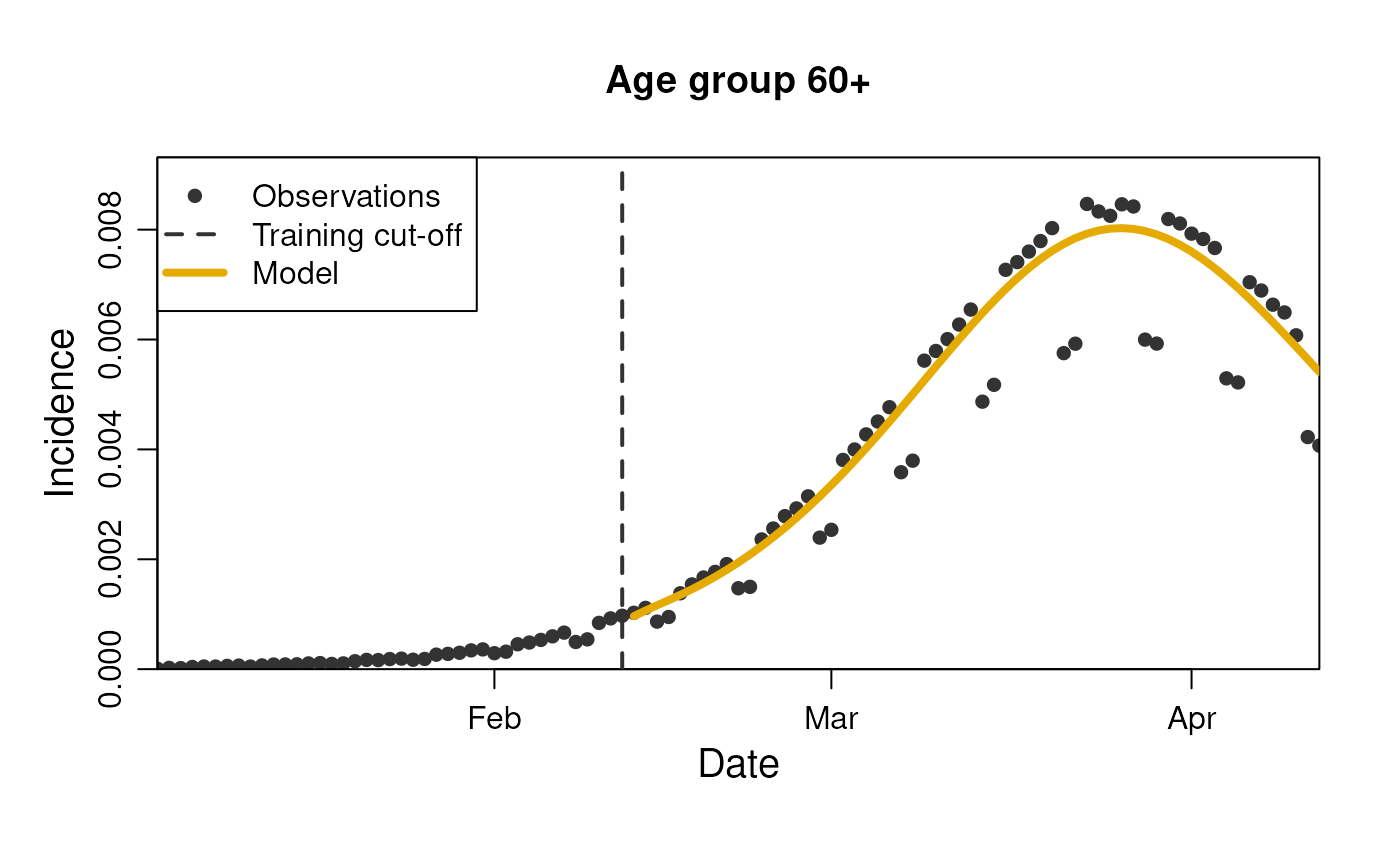
#> 9 2020-02-15 60+        0.00116               1      1

… and we can see the plots for each strata.

plot(
  model,
  observable = "incidence",
  prediction_length = 60,
  stratification = rlang::quos(age_group)
)

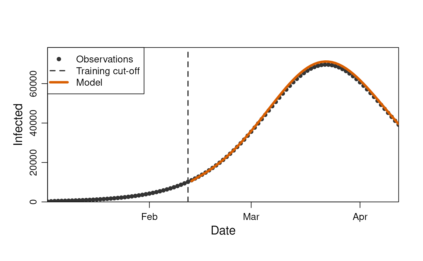
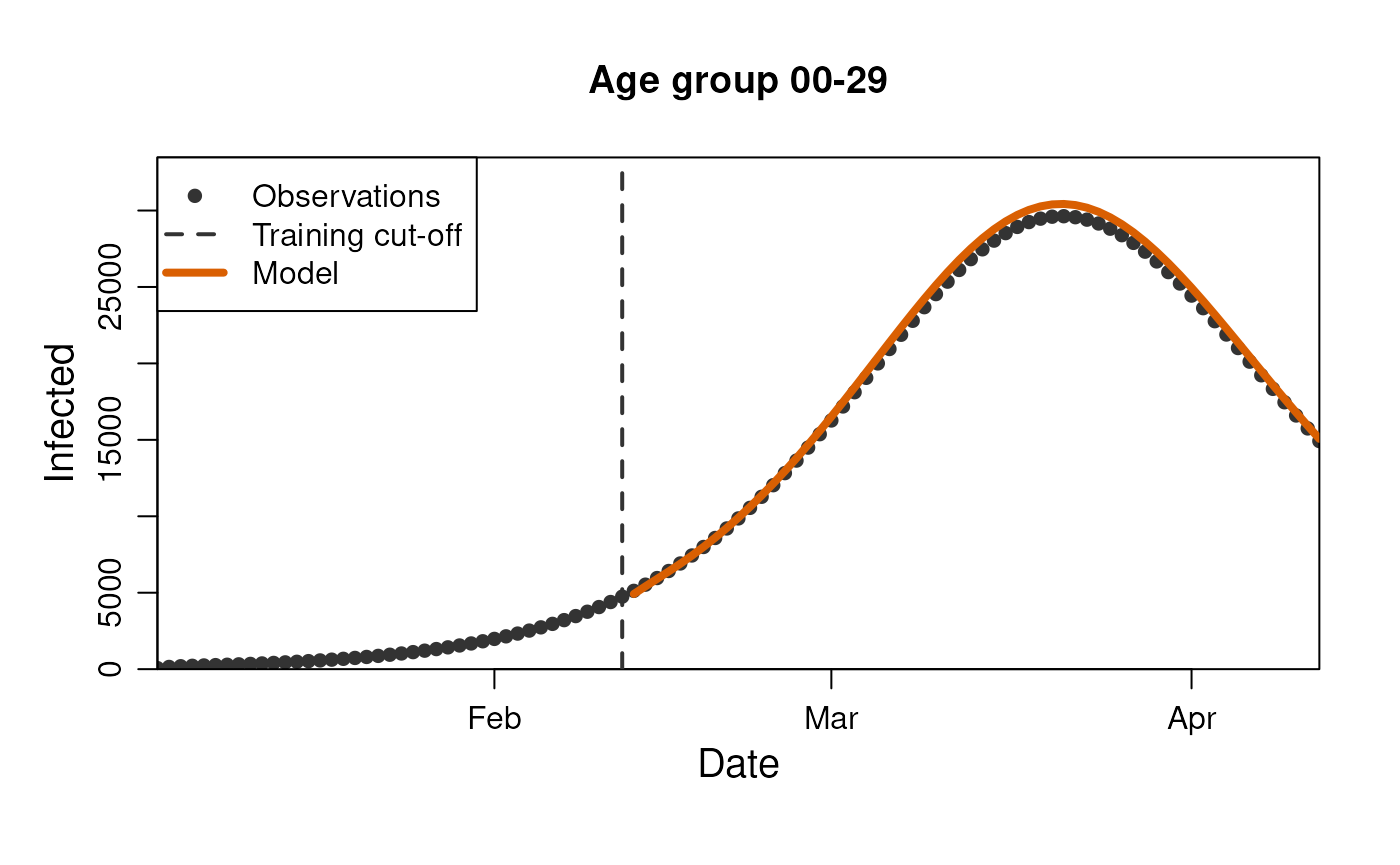
This can be done for all the observables we have mapped in the model.

model$get_results(
  observable = "n_infected",
  prediction_length = 5
)
#> # A tibble: 5 × 4
#>   date       n_infected realisation_id weight
#>   <date>          <dbl>          <dbl>  <dbl>
#> 1 2020-02-13     10575.              1      1
#> 2 2020-02-14     11643.              1      1
#> 3 2020-02-15     12685.              1      1
#> 4 2020-02-16     13731.              1      1
#> 5 2020-02-17     14818.              1      1

plot(
  model,
  observable = "n_infected",
  prediction_length = 60
)

model$get_results(
  observable = "n_infected",
  prediction_length = 3,
  stratification = rlang::quos(age_group)
)
#> # A tibble: 9 × 5
#>   date       age_group n_infected realisation_id weight
#>   <date>     <chr>          <dbl>          <dbl>  <dbl>
#> 1 2020-02-13 00-29          4917.              1      1
#> 2 2020-02-14 00-29          5415.              1      1
#> 3 2020-02-15 00-29          5902.              1      1
#> 4 2020-02-13 30-59          4198.              1      1
#> 5 2020-02-14 30-59          4614.              1      1
#> 6 2020-02-15 30-59          5024.              1      1
#> 7 2020-02-13 60+            1460.              1      1
#> 8 2020-02-14 60+            1614.              1      1
#> 9 2020-02-15 60+            1759.              1      1

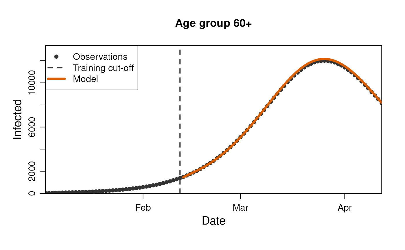
plot(
  model,
  observable = "n_infected",
  prediction_length = 60,
  stratification = rlang::quos(age_group)
)

model$get_results(
  observable = "n_positive",
  prediction_length = 5
)
#> # A tibble: 5 × 4
#>   date       n_positive realisation_id weight
#>   <date>          <dbl>          <dbl>  <dbl>
#> 1 2020-02-13      6874.              1      1
#> 2 2020-02-14      7568.              1      1
#> 3 2020-02-15      8246.              1      1
#> 4 2020-02-16      8925.              1      1
#> 5 2020-02-17      9632.              1      1

plot(
  model,
  observable = "n_positive",
  prediction_length = 60
)

model$get_results(
  observable = "n_positive",
  prediction_length = 3,
  stratification = rlang::quos(age_group)
)
#> # A tibble: 9 × 5
#>   date       age_group n_positive realisation_id weight
#>   <date>     <chr>          <dbl>          <dbl>  <dbl>
#> 1 2020-02-13 00-29          3196.              1      1
#> 2 2020-02-14 00-29          3520.              1      1
#> 3 2020-02-15 00-29          3836.              1      1
#> 4 2020-02-13 30-59          2729.              1      1
#> 5 2020-02-14 30-59          2999.              1      1
#> 6 2020-02-15 30-59          3266.              1      1
#> 7 2020-02-13 60+             949.              1      1
#> 8 2020-02-14 60+            1049.              1      1
#> 9 2020-02-15 60+            1144.              1      1

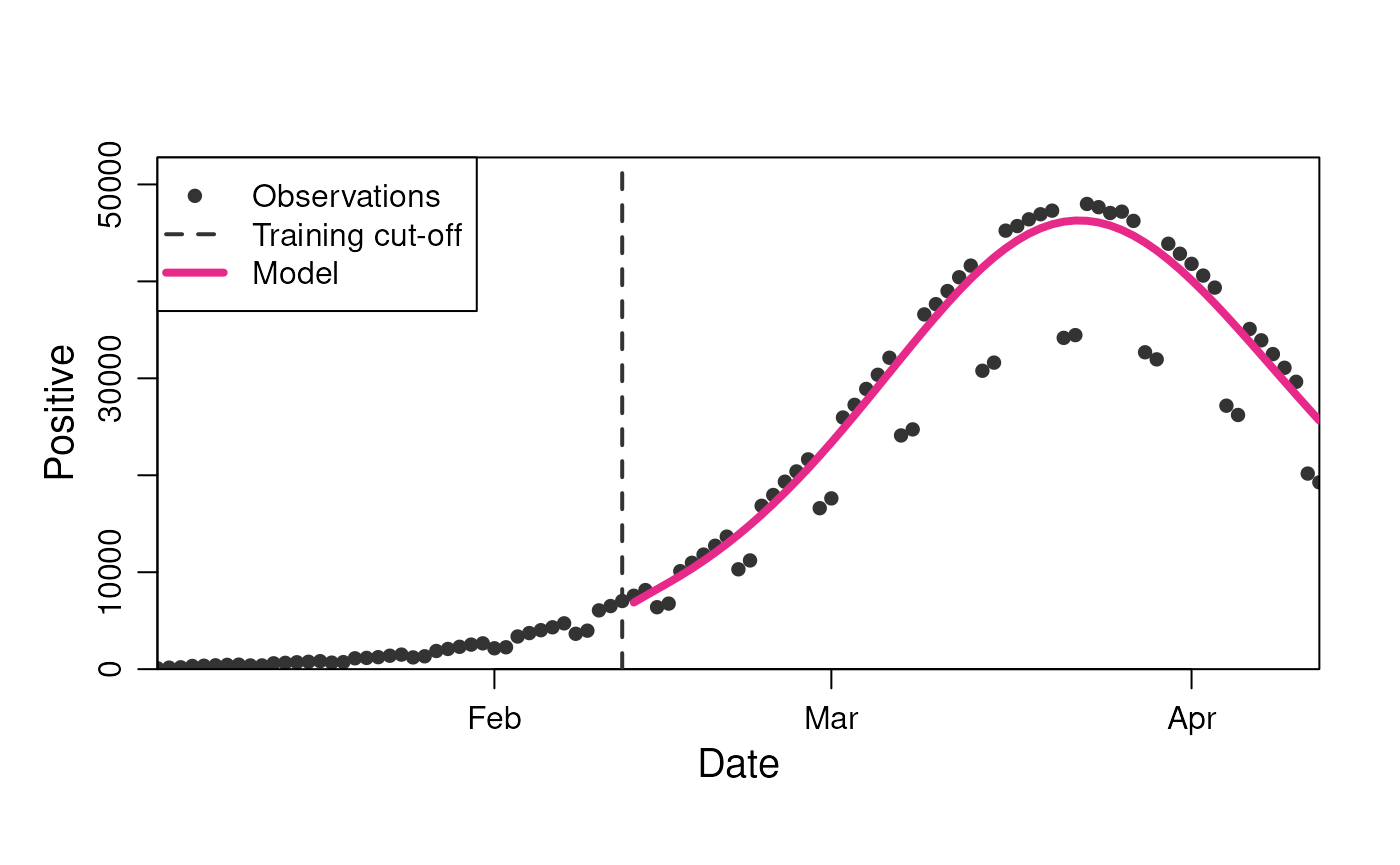
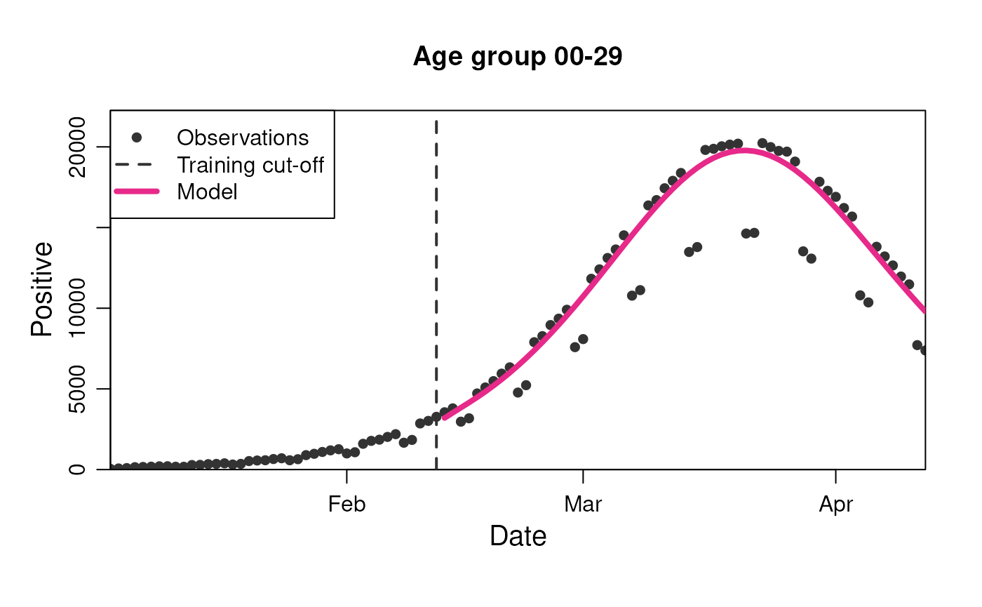
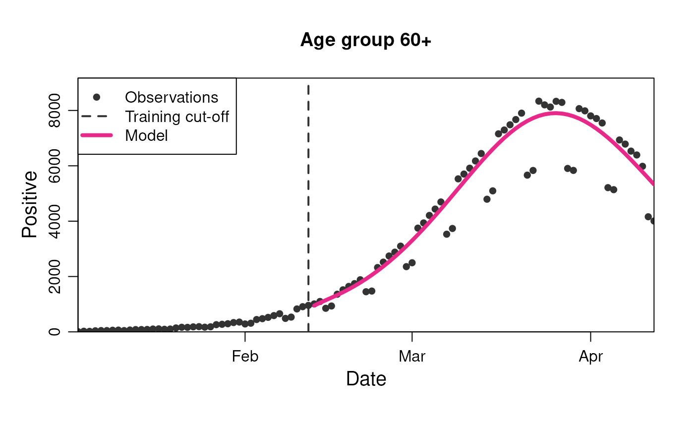
plot(
  model,
  observable = "n_positive",
  prediction_length = 60,
  stratification = rlang::quos(age_group)
)

model$get_results(
  observable = "n_admission",
  prediction_length = 5
)
#> # A tibble: 5 × 4
#>   date       n_admission realisation_id weight
#>   <date>           <dbl>          <dbl>  <dbl>
#> 1 2020-02-13        144.              1      1
#> 2 2020-02-14        166.              1      1
#> 3 2020-02-15        180.              1      1
#> 4 2020-02-16        194.              1      1
#> 5 2020-02-17        206.              1      1

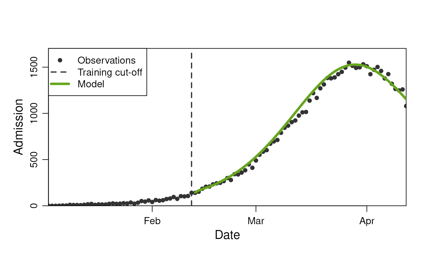
plot(
  model,
  observable = "n_admission",
  prediction_length = 60
)

model$get_results(
  observable = "n_admission",
  prediction_length = 3,
  stratification = rlang::quos(age_group)
)
#> # A tibble: 9 × 5
#>   date       age_group n_admission realisation_id weight
#>   <date>     <chr>           <dbl>          <dbl>  <dbl>
#> 1 2020-02-13 00-29            3.69              1      1
#> 2 2020-02-14 00-29            4.26              1      1
#> 3 2020-02-15 00-29            4.61              1      1
#> 4 2020-02-13 30-59           31.5               1      1
#> 5 2020-02-14 30-59           36.3               1      1
#> 6 2020-02-15 30-59           39.4               1      1
#> 7 2020-02-13 60+            108.                1      1
#> 8 2020-02-14 60+            125.                1      1
#> 9 2020-02-15 60+            136.                1      1

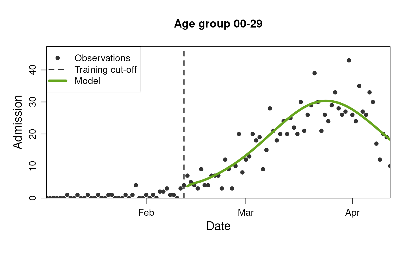
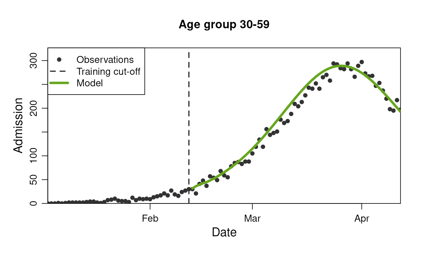
plot(
  model,
  observable = "n_admission",
  prediction_length = 60,
  stratification = rlang::quos(age_group)
)