A flexible SEIR model template

This class provides a diseasy model-template for a compartmental SEIR ordinary differential equation model. The number of consecutive exposed, infectious, and recovered compartments can flexibly be specified to generate a number of structurally different SEIR models.

Similarly, the number of age groups in the model can also be controlled to create structurally different models.

The model implements the following features:

A scaling of infection risk based on season (via DiseasySeason)
Contact matrices and activity scenarios (via DiseasyActivity)
Waning of immunity (via DiseasyImmunity)
Asymmetric cross-immunity interactions between variants (via DiseasyVariant)

See vignette(diseasy-model-ode-seir) for a detailed examples of how to use this model.

Value

A new instance of the DiseasyModelOdeSeir R6 class.

Super classes

diseasy::DiseasyBaseModule -> diseasy::DiseasyModel -> diseasy::DiseasyModelOde -> DiseasyModelOdeSeir

Active bindings

malthusian_scaling_factor: (numeric(1))
A scaling factor to apply to the contact matrices to account for structural differences in the model. Read only.

Methods

Public methods

DiseasyModelOdeSeir$new()
DiseasyModelOdeSeir$load_module()
DiseasyModelOdeSeir$get_results()
DiseasyModelOdeSeir$prepare_rhs()
DiseasyModelOdeSeir$set_forcing_functions()
DiseasyModelOdeSeir$malthusian_growth_rate()
DiseasyModelOdeSeir$initialise_state_vector()
DiseasyModelOdeSeir$rhs()
DiseasyModelOdeSeir$clone()

Inherited methods

Method `new()`

Creates a new instance of the DiseasyModelOdeSeir R6 class.

Usage

DiseasyModelOdeSeir$new(
  observables = FALSE,
  activity = TRUE,
  season = TRUE,
  variant = TRUE,
  immunity = TRUE,
  parameters = NULL,
  ...
)

Arguments

observables, activity, season, variant, immunity

(boolean or R6::R6Class instance)
If a boolean is given, it dictates whether to load a new instance module of this class.
If an instance of the module is provided instead, a copy of this instance is added to the DiseasyModel instance. This copy is a "clone" of the instance at the time it is added and any subsequent changes to the instance will not reflect in the copy that is added to DiseasyModel.

parameters

(named list())
List of parameters to set for the model during initialization.

Parameters controlling the structure of the model:

compartment_structure (named integer())
The structure of the compartments in the model. The names should be E, I, and R for the exposed, infectious, and recovered compartments, respectively. The exposed compartments can optionally be omitted.
age_cuts_lower (numeric())
Determines the age groups in the model.
malthusian_matching (logical(1))
Should the model be scaled such the Malthusian growth rate matches the corresponding SIR model?

Parameters controlling the dynamics of the model:

overall_infection_risk (numeric(1))
A scalar that scales contact rates to infection rates.
disease_progression_rates (named numeric())
The overall progression rates for the disease states. The reciprocal of each rate is the average time spent in the all of the corresponding compartments. The exposed compartments can optionally be omitted.

Parameters controlling initialisation routines

incidence_polynomial_order (integer(1))
The degree of the polynomial to fit to the incidence curves.
incidence_polynomial_training_length (integer(1))
The number of days to include in the incidence polynomial fit.
incidence_max_order_derivatives (integer(1))
The highest (informed) derivative from incidence data. Higher order derivatives are set to zero.

Parameters controlling the functional modules:

activity.weights (numeric(4))
Passed to ?DiseasyActivity$get_scenario_contacts(..., weights = activity.weights)
immunity.approximate_compartmental_args (named list())
Arguments passed to $approximate_compartmental()

Additional parameters are:

training_length (named numeric(3))
The number of days that should be included in the training splits of the data for the model. Allowed splits are: "training", "testing", and "validation".
incidence_feature_name (character(1))
The name of the observable that contains the incidence data to initialise from. * model_rate_to_observable (named list(named list(function(2))))
A named list of functions that maps the model rates to the observable in question (name). Each observable needs a map and reduce function contained in a list (the first nested list). The map function is applied in a dplyr::group_map() call and should take two arguments: - The first argument contains the model rate and information about group size: proportion and population. - The second argument contains the groups (stratification). The reduce function is applied in a dplyr::summarise() call to summarise across stratification levels. By default, the sum function is used and will work for all counting observables.

...

Parameters sent to DiseasyModel R6 constructor.

Method `load_module()`

Overload the $load_module() to re-initialise the helpers after loading

Usage

DiseasyModelOdeSeir$load_module(...)

Arguments

...: Arguments sent to parent method.

Method `get_results()`

The primary method used to request model results of a given observable at a given stratification

Usage

DiseasyModelOdeSeir$get_results(
  observable,
  prediction_length,
  quantiles = NULL,
  stratification = NULL
)

Arguments

observable: (character)
The observable to provide data or prediction for.
prediction_length: (numeric)
The number of days to predict. The prediction start is defined by last_queryable_date of the ?DiseasyObservables R6 class.
quantiles: (list(numeric))
If given, results are returned at the quantiles given.
stratification: (list(quosures) or NULL)
Use rlang::quos(...) to specify stratification. If given, expressions in stratification evaluated to give the stratification level.

Returns

A tibble tibble::tibble with predictions at the level specified by stratification level. In addition to stratification columns, the output has the columns:

- date (Date) specifying the date of the prediction.
- realisation_id (character) giving a unique id for each realization in the ensemble.
- weight (numeric) giving the weight of the realization in the ensemble.

Method `prepare_rhs()`

Allocate the helpers for the rhs method

Usage

DiseasyModelOdeSeir$prepare_rhs()

Method `set_forcing_functions()`

Set the forcing functions for the model.

Usage

DiseasyModelOdeSeir$set_forcing_functions(
  infected_forcing = NULL,
  state_vector_forcing = NULL
)

Arguments

infected_forcing: (function)
A function that takes arguments t and infected and modifies the number of infected at time t.
state_vector_forcing: (function)
A function that takes arguments t anddy_dt and modifies the flow into the compartments at time t.

Returns

NULL (called for side effects)

Method `malthusian_growth_rate()`

This function computes the Malthusian growth rate for the given model configuration.

Usage

DiseasyModelOdeSeir$malthusian_growth_rate(...)

Arguments

...: Parameters passed to $generator_matrix().

Details

This section follows the method outlined in doi: 10.1098/rsif.2009.0386 To compute the scaling, we need to compute the Jacobian matrix of the linearised system. Here, we linearise around S = 1. In this limit, there is no interaction with variants (since everyone is susceptible). The Malthusian growth rate is therefore not dependent on factors such as cross-immunity.

Returns

(numeric(1))
The Malthusian growth rate for the model.

Method `initialise_state_vector()`

Infer the state_vector from incidence data

Usage

DiseasyModelOdeSeir$initialise_state_vector(
  incidence_data,
  overall_infection_risk = self %.% parameters %.% overall_infection_risk,
  ei_rs_balance = 1,
  method = c("derivative", "eigen-value")
)

Arguments

incidence_data

incidence_data (data.frame)
Incidence observations as a data.frame with columns - date: The date of the observations - age_group: The age group of the incidence observation (following diseasystore::age_labels() format) - variant: The variant of the incidence observation. - incidence: The incidence in the age group at the given date

overall_infection_risk

(numeric)
The overall multiplier for the infection risk for the model.

ei_rs_balance

(numeric(1))
Which estimate should be priorities when normalising? See details.

method

(character(1))
The method to use for initialising the state vector.

derivative: Directly infers the EI compartments from derivatives of the incidence signal.
eigen-value: Uses the eigenvalues of the generator matrix to infer the state vector.

See the article SEIR-initialisation in the online documentation for more information.

Details

The inference of the state_vector from incidence data is two-fold: EI states are inferred with one method and the RS states are inferred with another. The methods are described in detail in the initialisation article vignette("SEIR-initialisation").

When these estimates are combined, there is a degree of freedom in how to weight the estimates when normalising the state vector. This is controlled by the ei_rs_balance parameter. If ei_rs_balance = 1, the estimate for EI states are prioritised, and only the RS states are modified. If ei_rs_balance = 0, the estimate for RS states are prioritised.

Returns

(numeric())
The initial state vector for the model (invisibly).

Method `rhs()`

The vectorised right hand side (RHS) function of the system of differential equations

Usage

DiseasyModelOdeSeir$rhs(
  t,
  state_vector,
  parms = NULL,
  overall_infection_risk = self %.% parameters %.% overall_infection_risk
)

Arguments

t: (numeric(1))
The time to solve for.
state_vector: (numeric())
The state vector to compute the RHS from.
parms: (list)
Argument to comply with deSolve::ode format. Not used.
overall_infection_risk: (numeric)
The overall multiplier for the infection risk for the model.

Returns

(numeric())
The rate of change for the differential equations.

Method `clone()`

The objects of this class are cloneable with this method.

Usage

DiseasyModelOdeSeir$clone(deep = FALSE)

Arguments

deep: Whether to make a deep clone.

Examples

  # The model can be instantiated almost without arguments, but
  # to illustrate its use, we configure a simple model:

  # First, we add a observables modules with example data bundled
  # with the package.
  obs <- DiseasyObservables$new(
    diseasystore = DiseasystoreSeirExample,
    conn = DBI::dbConnect(duckdb::duckdb())
  )

  # The observables module also defines the time if interest via
  # the `last_queryable_date` field. Data before this date are
  # used to train the models, and predictions start on this date.
  obs$set_last_queryable_date(as.Date("2020-02-29"))

  # Define the incidence data to initialise the model
  obs$define_synthetic_observable(
    name = "incidence",
    mapping = \(n_positive, n_population) n_positive / (n_population * 0.65)
  )

  # The example data uses a simple activity scenario for Denmark,
  # which we replicate here
  act <- DiseasyActivity$new(contact_basis = contact_basis$DK)
  act$set_activity_units(dk_activity_units)
  act$change_activity(date = as.Date("2020-01-01"), opening = "baseline")

  # We create a simple model instance
  m <- DiseasyModelOdeSeir$new(
    observables = obs,
    activity = act,
    parameters = list(
      "age_cuts_lower" = c(0, 30, 60),
      "overall_infection_risk" = 0.025,
      "disease_progression_rates" = c("E" = 1 / 2, "I" = 1 / 4)
    )
  )

  # Run the model to predict incidence
  prediction <- m$get_results("incidence", prediction_length = 30)
  print(head(prediction, 5))
#> # A tibble: 5 × 4
#>   date       incidence realisation_id weight
#>   <date>         <dbl>          <dbl>  <dbl>
#> 1 2020-03-01   0.00530              1      1
#> 2 2020-03-02   0.00549              1      1
#> 3 2020-03-03   0.00568              1      1
#> 4 2020-03-04   0.00586              1      1
#> 5 2020-03-05   0.00603              1      1

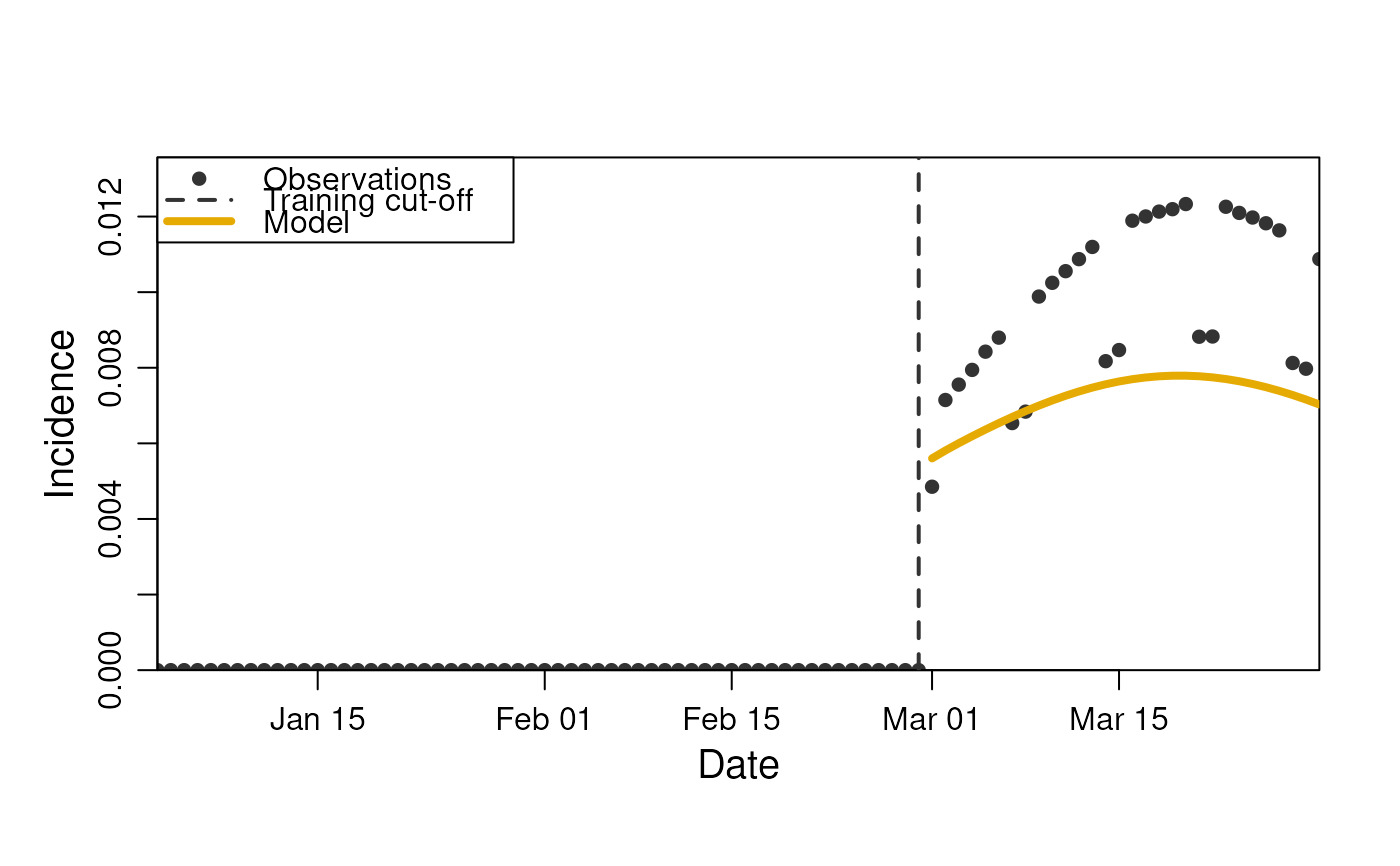
  # Plot the results
  plot(m, observable = "incidence", prediction_length = 30)


  rm(m, act, obs)

Value

See also

Super classes

Active bindings

Methods

Public methods

Method new()

Usage

Arguments

Method load_module()

Usage

Arguments

Method get_results()

Usage

Arguments

Returns

Method prepare_rhs()

Usage

Method set_forcing_functions()

Usage

Arguments

Returns

Method malthusian_growth_rate()

Usage

Arguments

Details

Returns

Method initialise_state_vector()

Usage

Arguments

Details

Returns

Method rhs()

Usage

Arguments

Returns

Method clone()

Usage

Arguments

Examples

Method `new()`

Method `load_module()`

Method `get_results()`

Method `prepare_rhs()`

Method `set_forcing_functions()`

Method `malthusian_growth_rate()`

Method `initialise_state_vector()`

Method `rhs()`

Method `clone()`