DiseasyRegions • diseasy

library(diseasy)
#> Loading required package: diseasystore
#> 
#> Attaching package: 'diseasy'
#> The following object is masked from 'package:diseasystore':
#> 
#>     diseasyoption

Overview

The DiseasyRegions module defines the regional scope for the models. In addition, it provides a common place to define the demography available for those regions, and the adjacency between regions.

The module is intentionally generic. Region identifiers are treated as ordinary character values and are matched exactly. This means that, e.g., the region "north" is not interpreted as a parent of "north_subregion".

Data structure

DiseasyRegions uses three inputs:

regions: a character vector defining the selected region scope.
demography: a data.frame with one region column, optional stratification columns, and one population column.
adjacency: a data.frame describing connectedness between pairs of regions (see the Regional adjacency section for further details).

The demography data must include the columns region and population. Any additional columns are treated as stratification variables.

all_regions <- c("north", "south", "east", "north_subregion")

demography <- data.frame(
  region = rep(all_regions, each = 2),
  age_group = rep(c("0-17", "18+"), times = length(all_regions)),
  population = c(
    100000, 250000,
    80000, 180000,
    60000, 140000,
    20000, 50000
  )
)

demography
#>            region age_group population
#> 1           north      0-17     100000
#> 2           north       18+     250000
#> 3           south      0-17      80000
#> 4           south       18+     180000
#> 5            east      0-17      60000
#> 6            east       18+     140000
#> 7 north_subregion      0-17      20000
#> 8 north_subregion       18+      50000

The adjacency data must include exactly the columns from, to, and adjacency. The from and to columns should contain the same set of region identifiers.

adjacency <- tidyr::expand_grid(
  from = all_regions,
  to = all_regions
)

adjacency[["adjacency"]] <- 0.1
adjacency[adjacency$from == adjacency$to, "adjacency"] <- 1
adjacency[adjacency$from == "north" & adjacency$to == "south", "adjacency"] <- 0.5
adjacency[adjacency$from == "south" & adjacency$to == "north", "adjacency"] <- 0.5

adjacency
#> # A tibble: 16 × 3
#>    from            to              adjacency
#>    <chr>           <chr>               <dbl>
#>  1 north           north                 1  
#>  2 north           south                 0.5
#>  3 north           east                  0.1
#>  4 north           north_subregion       0.1
#>  5 south           north                 0.5
#>  6 south           south                 1  
#>  7 south           east                  0.1
#>  8 south           north_subregion       0.1
#>  9 east            north                 0.1
#> 10 east            south                 0.1
#> 11 east            east                  1  
#> 12 east            north_subregion       0.1
#> 13 north_subregion north                 0.1
#> 14 north_subregion south                 0.1
#> 15 north_subregion east                  0.1
#> 16 north_subregion north_subregion       1

Regional adjacency

DiseasyRegions builds on the concept of a degree of “connectedness” between the different regions. Here, this “connectedness” is referred to as “adjacency” in alignment with other models.

Different measures for adjacency can be extracted from real-world data which have very different interpretations. Adjacency is often described from information about “movement” such as mobility data or surveys on how people move between regions. Alternatively adjacency can be derived from “infection” data such as genetic phylogeny.

While these seem very similar, there are substantial differences in how these adjacencies are expressed numerically, and how they should be implemented in disease spread models. Our framework assumes a reality where disease is transported between regions by people returning to their own region (travel or commuting), that is: there is no immigration or emigration. If the supplied adjacency describes a movement matrix it is furthermore assumed that people travelling to a place transmits disease equally with people travelling from a place. Which in turns means that the resulting infection matrix used in the models will be symmetric.

In diseasy, the adjacency of DiseasyRegions are implemented in SEIR-like models and it helps to be clear on how this adjacency is used to illustrate these differences.

To begin, let’s define the “movement matrix” $\Phi$ between $R$ connected regions:

$\overline{\overline{\Phi}} = \begin{bmatrix} \phi_{1,1} & \cdots & \phi_{1,R} \\ \vdots & \ddots & \vdots \\ \phi_{R,1} & \cdots & \phi_{R,R} \end{bmatrix}$

If we interpret these adjacencies as “the average fraction of contacts between regions”, we can diagram the SEIR compartments of a two-region model as:

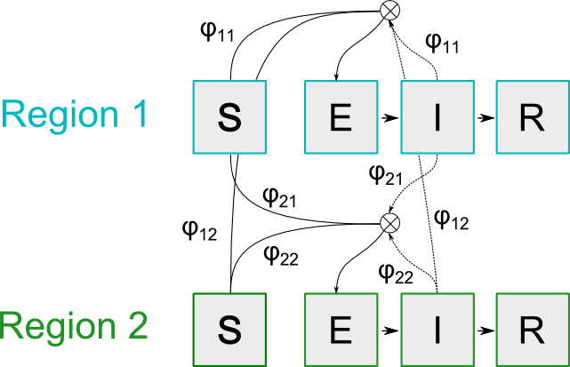
SEIR model overview for a two region model

With the following equations for the infectious compartments in region $1$ $\dot{I}_1 = \beta\left( \underbrace{S_1 \phi_{1,1}}_\textrm{stay} \underbrace{\phi_{1,1} I_1}_\textrm{stay} + \underbrace{S_1 \phi_{1,1}}_\textrm{stay} \underbrace{\phi_{1,2} I_2}_\textrm{travel} + \underbrace{S_1 \phi_{2,1}}_\textrm{travel}\underbrace{\phi_{2,2} I_2}_\textrm{stay} + \underbrace{S_1 \phi_{2,1}}_\textrm{travel}\underbrace{\phi_{2,1} I_1}_\textrm{travel}\right) - r_I I_1$ where we divide the types of contacts into whether individuals stay in their own region or travel¹ to other regions.

In general, we can express the dynamics in matrix form assuming $R$ different regions $\dot{\overline{I}} = \beta\overline{S}\circ\overline{\overline{\Theta}}\cdot\overline{I} - r_I \overline{I}$

Where $\circ$ is the Hadamard product (element-wise multiplication).

The matrix elements of $\overline{\overline{\Theta}}$ contains the probability that individual interact across regions, with elements $\Theta_{x,y} = \sum_z \phi_{z,x} \phi_{z,y}$ .

These elements compute the probability that individuals in region $x$ travel to region $z$ AND individuals in region $y$ travel to region $z$ .

For the 2-region system, the mixing can be expressed in matrix form as: $\overline{\overline{\Theta}} = \begin{bmatrix} \phi_{1,1}^2 + \phi_{2,1}^2 & \phi_{1,1}\phi_{1,2} + \phi_{2,1}\phi_{2,2} \\ \phi_{2,2}\phi_{2,1} + \phi_{1,2}\phi_{1,1} & \phi_{2,2}^2 + \phi_{1,2}^2 \end{bmatrix}$

In this formalism, the $\Theta$ which satisfies: $\dot{I} = \dot{I}_1 + \dot{I}_2 = \beta S I - r_I I$

requires $\overline{S}\cdot\overline{\overline{\Theta}}\cdot\overline{I} = S I$

That leads to the following expression: $$ S_1 (\phi_{1,1}^2 + \phi_{2,1}^2) I_1 + S_1 (\phi_{1,1}\phi_{1,2} + \phi_{2,1}\phi_{2,2}) I_2 + \\ S_2 (\phi_{2,2}^2 + \phi_{1,2}^2) I_2 + S_2 (\phi_{2,2}\phi_{2,1} + \phi_{1,2}\phi_{1,1}) I_1 $$

If we assume there is no spatial structure and therefore all matrix elements are identical: $\phi_{x,y} = \phi$

Then we can reduce the expression $\Rightarrow S_1 (2\phi^2) I_1 + S_1 (2\phi^2) I_2 + S_2 (2\phi^2) I_2 + S_2 (2\phi^2) I_1$

$\Rightarrow S_1 (2\phi^2) (I_1 + I_2) + S_2 (2\phi^2) (I_1 + I_2)$

$\Rightarrow (2\phi^2) (S_1 + S_2) (I_1 + I_2)$

$\Rightarrow (2\phi^2) S I$

Which means that the neutral matrix elements for the 2-region system are: $\phi = \frac{1}{\sqrt{2}}$

and in general for the n-region system²: $\phi = \frac{1}{\sqrt{n}}$

This “movement matrix” $\overline{\overline{\Phi}}$ can be estimated from information on how individuals travel, such as from survey or mobility data.

Alternatively, we can consider the $\overline{\overline{\Theta}}$ matrix which we can think of as a “infection-flow” matrix. This matrix identifies the flow of infections from individuals residing in regions $x$ to individuals residing in regions $y$ . Such matrix may be estimated from more direct measurements of disease flow such as from genetic data or contact tracing.

The $\Phi$ matrix will be normalised such that its row sums are 1.

DiseasyRegions can take either type of adjacency matrix.

The stored adjacency input is long form, but the module also exposes an $infection_flow_matrix field. This field returns a matrix representation of adjacency for the currently selected regions.

The matrix is derived in three steps:

the stored adjacency data are filtered to the selected regions;
the matrix is normalised so that row sums are 1.

Creating a regional module

A DiseasyRegions object can be created and then configured with the selected regions, demography, and adjacency data. Each setter validates the candidate input before storing it.

region <- DiseasyRegions$new()

region
#> # DiseasyRegions #############################################
#> Regions: No regions have been specified
#> Total population: No population data loaded
#> Theta matrix: No adjacency data loaded

region$set_regions(regions = c("north", "south", "east"))
region$set_demography(demography = demography)
region$set_adjacency(adjacency = adjacency)

region
#> # DiseasyRegions #############################################
#> Regions: east, north, south
#> Total population: 810000
#> Theta matrix: Max eigenvalue 1

The $demography field returns demography filtered to the currently selected regions.

region %.% demography
#>   region age_group population
#> 1   east      0-17      60000
#> 2   east       18+     140000
#> 3  north      0-17     100000
#> 4  north       18+     250000
#> 5  south      0-17      80000
#> 6  south       18+     180000

Population totals can be computed directly from the filtered demography.

aggregate(
  population ~ region,
  data = region %.% demography,
  FUN = sum
)
#>   region population
#> 1   east     200000
#> 2  north     350000
#> 3  south     260000

The active bindings $adjacency and $infection_flow_matrix expose derived views of adjacency input after filtering to the selected regions.

region %.% adjacency
#> # A tibble: 9 × 3
#>   from  to    adjacency
#>   <chr> <chr>     <dbl>
#> 1 east  east        1  
#> 2 east  north       0.1
#> 3 east  south       0.1
#> 4 north east        0.1
#> 5 north north       1  
#> 6 north south       0.5
#> 7 south east        0.1
#> 8 south north       0.5
#> 9 south south       1

region %.% infection_flow_matrix
#>            east     north     south
#> east  0.7083333 0.1302083 0.1302083
#> north 0.1302083 0.4921875 0.3945312
#> south 0.1302083 0.3945312 0.4921875

Changing the selected regions

The selected regional scope can be changed with $set_regions(). The new regions must be available in the stored adjacency and demography data.

region$set_regions(regions = c("north", "south"))

region %.% regions
#> [1] "north" "south"

The active fields now reflect the updated scope.

region %.% demography
#>   region age_group population
#> 1  north      0-17     100000
#> 2  north       18+     250000
#> 3  south      0-17      80000
#> 4  south       18+     180000

region %.% adjacency
#> # A tibble: 4 × 3
#>   from  to    adjacency
#>   <chr> <chr>     <dbl>
#> 1 north north       1  
#> 2 north south       0.5
#> 3 south north       0.5
#> 4 south south       1

region %.% infection_flow_matrix
#>           north     south
#> north 0.5555556 0.4444444
#> south 0.4444444 0.5555556

Exact matching

The generic module does not use hierarchical matching. In the example data, "north" and "north_subregion" are two different region identifiers.

region$set_regions(regions = "north")

region %.% demography
#>   region age_group population
#> 1  north      0-17     100000
#> 2  north       18+     250000

The result includes rows for "north", but not for "north_subregion".

Updating demography and adjacency

The demography and adjacency can also be updated after the module has been created. Candidate data are validated before they are stored, so an invalid update leaves the existing object state unchanged.

demography_new <- demography
demography_new[
  demography_new[["region"]] == "north" & demography_new[["age_group"]] == "18+",
  "population"
] <- 260000

region$set_demography(demography = demography_new)

region %.% demography
#>   region age_group population
#> 1  north      0-17     100000
#> 2  north       18+     260000

adjacency_new <- adjacency
adjacency_new[
  adjacency_new[["from"]] == "north" & adjacency_new[["to"]] == "south",
  "adjacency"
] <- 0.75
adjacency_new[
  adjacency_new[["from"]] == "south" & adjacency_new[["to"]] == "north",
  "adjacency"
] <- 0.75

region$set_regions(regions = c("north", "south"))
region$set_adjacency(adjacency = adjacency_new)

region %.% adjacency
#> # A tibble: 4 × 3
#>   from  to    adjacency
#>   <chr> <chr>     <dbl>
#> 1 north north      1   
#> 2 north south      0.75
#> 3 south north      0.75
#> 4 south south      1

Validation

The module checks that selected regions are available in the stored demography and adjacency. For example, trying to select a region that is not present in the data will fail.

try(region$set_regions(regions = "west"))
#> Error in base::tryCatch(base::withCallingHandlers({ : 
#>   1 assertions failed:
#>  * Variable 'regions': Must be a subset of
#>  * {'east','north','north_subregion','south'}, but has additional
#>  * elements {'west'}.

The adjacency data must also contain the same region identifiers in the from and to columns.

bad_adjacency <- data.frame(
  from = c("north", "south"),
  to = c("south", "east"),
  adjacency = c(1, 1)
)

try(region$set_adjacency(adjacency = bad_adjacency))
#> Error in base::tryCatch(base::withCallingHandlers({ : 
#>   2 assertions failed:
#>  * `adjacency` incomplete: All two-way connections between regions must
#>  * be specified!
#>  * Variable 'self %.% regions': Must be a subset of {'south','east'},
#>  * but has additional elements {'north'}.