Scoring and fitting models and ensembles • diseasy

Introduction

Every model in diseasy contains some parameterisation of its forecasts. These parameters can then be optimised to align model forecasts with the real-world observations.

This operation requires only two components: 1) A metric for the optimiser to optimise 2) Free parameters for the optimiser to control

Model parameterisation

Models diseasy will contain parameters that are either specific to the model (e.g. the compartment structure in ?DiseasyModelOdeSeir) or parameters meant to control the functional modules passed to the model (e.g. ?DiseasySeason).

For example, lets consider the parameters of ?DiseasyModelG0:

model <- DiseasyModelG0$new()
model$parameters
#> $training_length
#>   training    testing validation 
#>          7          0          0 
#> 
#> $season.scale
#> NULL
#> 
#> $season.peak
#> NULL
#> 
#> $seed
#> [1] 0
#> 
#> $n_realisations
#> [1] 100

This model has parameters inherent to the model and parameters related to the season module. This latter type of parameters, parameters that should modify the internal modules are treated specially: If these parameters are NULL they will inherit the defaults (if any) from the module. If they are different from NULL they will be applied to the module.

A couple of examples:

# We create a default season module which includes a "no seasonality" scenario
# with no parameters
season <- DiseasySeason$new(reference_date = Sys.Date())

model <- DiseasyModelG0$new(season = season)
print(model$parameters)
#> $training_length
#>   training    testing validation 
#>          7          0          0 
#> 
#> $season.scale
#> NULL
#> 
#> $season.peak
#> NULL
#> 
#> $seed
#> [1] 0
#> 
#> $n_realisations
#> [1] 100


# If we change to the "covid_season_v1" season model, we have a single "scale"
# parameter in the season model
season$use_covid_season_v1()

model <- DiseasyModelG0$new(season = season)
print(model$parameters) # ... and this scale is copied to the model
#> $training_length
#>   training    testing validation 
#>          7          0          0 
#> 
#> $season.scale
#> [1] 0.4825524
#> 
#> $season.peak
#> NULL
#> 
#> $seed
#> [1] 0
#> 
#> $n_realisations
#> [1] 100


# If we change to the "cosine_Season" season model, we have both a "scale"
# parameter and a "peak" parameter in the season model
season$use_cosine_season()

model <- DiseasyModelG0$new(season = season)
print(model$parameters) # ... and these are copied to the model
#> $training_length
#>   training    testing validation 
#>          7          0          0 
#> 
#> $season.scale
#> [1] 0.5726693
#> 
#> $season.peak
#> [1] 20.09946
#> 
#> $seed
#> [1] 0
#> 
#> $n_realisations
#> [1] 100


# If we provide specific values to the model, then these values are
# passed to the season module.
model <- DiseasyModelG0$new(
  season = season,
  parameters = list("season.scale" = 0.5)
)
print(model$parameters) # "peak" value is still copied
#> $training_length
#>   training    testing validation 
#>          7          0          0 
#> 
#> $season.scale
#> [1] 0.5
#> 
#> $season.peak
#> [1] 20.09946
#> 
#> $seed
#> [1] 0
#> 
#> $n_realisations
#> [1] 100
print(attr(model$season$model, "dots"))
#> NULL

Marking parameters for optimisation

Any parameter set to NA is considered to be “marked for optimisation” meaning that the fitting routine will attempt to estimate the parameter under the scoring metric.

The default value for the parameter is stored as an attribute on any NA parameter and will be used as the starting point for the optimisation.

model <- DiseasyModelG0$new(
  season = season,
  parameters = list("season.scale" = NA) # Mark for optimisation
)
print(model$parameters[["season.scale"]])
#> [1] NA
#> attr(,"default")
#> [1] 0.5726693

The starting point for optimisation and the parameter range of optimisation can be set by modifying the “default” and “range” attributes. For this purpose, we provide the helper function set_attributes to modify the attributes inline.

The range can either be : - unbounded c(NA, NA) (the default) - bounded from a single direction c(min_value, NA) or c(NA, max_value) - bounded from both directions c(min_value, max_value)

model <- DiseasyModelG0$new(
  season = season,
  parameters = list(
    "season.scale" = set_attributes(
      NA, # Mark for optimisation
      list("default" = 0.25, "range" = c(0, 0.5)) # Control the optimisation
    )
  )
)
print(model$parameters[["season.scale"]])
#> [1] NA
#> attr(,"default")
#> [1] 0.25
#> attr(,"range")
#> [1] 0.0 0.5

Updating parameters

The parameters can either be set during the initialisation of the model as we have seen above:

model <- DiseasyModelG0$new(
  season = season,
  parameters = list("season.scale" = 0.25)
)
print(model$parameters["season.scale"])
#> $season.scale
#> [1] 0.25

But the parameters can also be modified after initialisation via the $update_parameters() method:

model$update_parameters(list("season.scale" = 0.7))
print(model$parameters["season.scale"])
#> $season.scale
#> [1] 0.7

The scoring metric

The principal metric used in diseasy is the likelihood which compares the model forecast with observations for each time-point at each strata and computes the mean likelihood across the strata for the given time-point.

Different observation have different distributions and therefore diseasy supports multiple methods for computing the likelihood given the underlying (assumed) distribution.

The scoring of the forecasts are controlled by the ?DiseasyScoring module, where users can define the scoring metric and which includes a method to compute the likelihood for a given set of model trajectories (i.e. the output from $get_results()).

scoring <- DiseasyScoring$new()

scoring
#> # DiseasyScoring #############################################
#> Observation noise model: poisson

The scoring metric can be controlled with the $set_noise_model() method:

scoring$set_noise_model("negative binomial", overdispersion = 2)

scoring
#> # DiseasyScoring #############################################
#> Observation noise model: negative binomial with overdispersion 2

With the scoring metric defined, we can compute the likelihood for a set of model trajectories with $compute_likelihood():

observables <- DiseasyObservables$new(
  diseasystore = "simulist",
  conn = \() DBI::dbConnect(duckdb::duckdb(), ":memory:")
)
#> duckdb keeps downloaded extensions and secrets in a temporary directory:
#> ℹ /tmp/RtmpwYxxo1/duckdb
#> This is removed when the R session ends.
#> • Extensions are re-downloaded each session.
#> • Secrets are lost.
#> ℹ Run duckdb(shared_home = TRUE) (or create ~/.duckdb) to keep them (suitable for most users).
#> ℹ Run duckdb(shared_home = FALSE) to accept the temporary directory (and silence this message).
#> ℹ See ?duckdb_storage for details and alternatives.

observables$set_last_queryable_date(as.Date("2020-03-01"))

model <- DiseasyModelG0$new(
  observables = observables
)

trajectories <- model$get_results(observable = "n_admission", prediction_length = 7)

model$scoring$compute_likelihood(trajectories)
#> # A tibble: 100 × 3
#>    realisation_id weight negative_log_likelihood
#>    <chr>           <dbl>                   <dbl>
#>  1 1                   1                    32.4
#>  2 10                  1                    32.7
#>  3 100                 1                    34.0
#>  4 11                  1                    34.9
#>  5 12                  1                    34.1
#>  6 13                  1                    35.3
#>  7 14                  1                    34.1
#>  8 15                  1                    32.0
#>  9 16                  1                    32.9
#> 10 17                  1                    34.1
#> # ℹ 90 more rows

Fitting parameters

With the free parameters identified and the scoring metric defined, we can use the $fit() method to optimise the free parameters using the “testing” data window.

# Generate model to fit
observables <- DiseasyObservables$new(
  diseasystore = DiseasystoreSeirExample,
  conn = \() DBI::dbConnect(duckdb::duckdb(), ":memory:")
)
#> duckdb keeps downloaded extensions and secrets in a temporary directory:
#> ℹ /tmp/RtmpwYxxo1/duckdb
#> This is removed when the R session ends.
#> • Extensions are re-downloaded each session.
#> • Secrets are lost.
#> ℹ Run duckdb(shared_home = TRUE) (or create ~/.duckdb) to keep them (suitable for most users).
#> ℹ Run duckdb(shared_home = FALSE) to accept the temporary directory (and silence this message).
#> ℹ See ?duckdb_storage for details and alternatives.
observables$set_last_queryable_date(as.Date("2020-03-01"))

# Define the incidence from the example data
mapping <- \(n_infected, n_population) n_infected / n_population
observables$define_synthetic_observable("incidence", mapping)

# Generate a modified model of the "true" generating model
# with a specified "testing" window
model <- generate_example_seir_model(
  module_overrides = list(
    "observables" = observables
  ),
  parameter_overrides = list(
    "training_length" = c("training" = 21, "testing" = 7, "validation" = 0)
  )
)

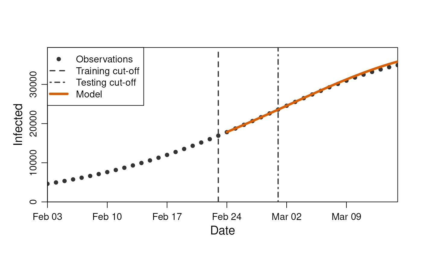
We can see the prediction using the default parameters

model$plot(observable = "n_infected", prediction_length = 14)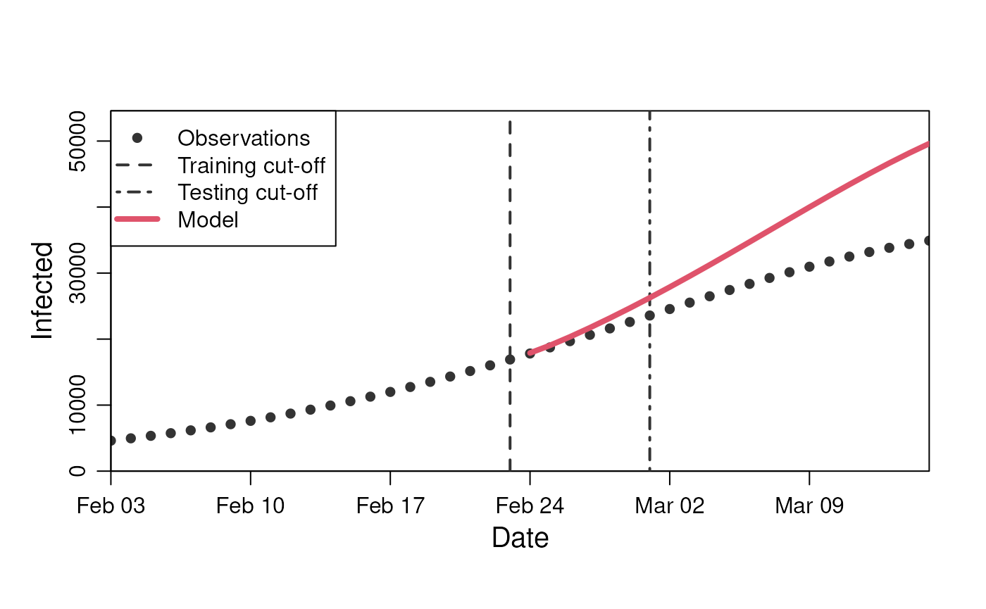

# The default model does not currently include the scoring module, so we
# manually load
model$load_module(scoring)

# Mark the overall infection risk for fitting
model$update_parameters(list("overall_infection_risk" = NA))

# Estimate free parameters
model$fit(observable = "n_infected")

# Show estimated parameters
model$parameters["overall_infection_risk"]
#> $overall_infection_risk
#> [1] 0.02330102

model$plot(observable = "n_infected", prediction_length = 14)